Judgment and Decision Making, vol. 1, no. 1, July 2006, pp. 1-12.
Biases in casino betting: The hot hand and the gambler's fallacy
James Sundali1
Managerial Sciences
University of Nevada, Reno,
Rachel Croson
Operations and Information Management
Wharton School
University of Pennsylvania
Abstract
We examine two departures of individual perceptions of
randomness from probability theory: the hot hand and the
gambler's fallacy, and their respective opposites. This
paper's first contribution is to use data from the field
(individuals playing roulette in a casino) to demonstrate the
existence and impact of these biases that have been previously
documented in the lab. Decisions in the field are consistent
with biased beliefs, although we observe significant individual
heterogeneity in the population. A second contribution is to
separately identify these biases within a given individual,
then to examine their within-person correlation. We find a
positive and significant correlation across individuals between
hot hand and gambler's fallacy biases, suggesting a common
(root) cause of the two related errors. We speculate as to the
source of this correlation (locus of control), and suggest
future research which could test this speculation.
Keywords: judgment and decision making, hot hand, gambler's fallacy,
casino betting, field data, roulette
1 Introduction
Almost every decision we make involves uncertainty in some way. Yet
research on decision making under uncertainty demonstrates that our
judgments are often not consistent with probability theory. Intuitive
ideas of randomness depart systematically from the laws of chance.
This research suggests that we have developed a number of judgment
heuristics for analyzing complex, real-world events. Although many
decisions based on these heuristics are consistent with probability
theory, there are also situations where heuristics lead to statistical
illusions and suboptimal actions.
This paper investigates the existence and impact of two of these
statistical illusions; the gambler's fallacy and the
hot hand. Both of these illusions characterize individuals'
perceptions of non-autocorrelated random sequences. Thus both involve
perceptions of sequences of events rather than one-time events.
The gambler's fallacy is a belief in negative autocorrelation of a
non-autocorrelated random sequence of outcomes like coin flips. For
example, imagine Jim repeatedly flipping a (fair) coin and guessing the
outcome before it lands. If he believes in the gambler's fallacy, then
after observing three heads in a row, his subjective probability of
seeing another head is less than 50%. Thus he believes a tail is
"due," and is more likely to appear on the next flip than a head.
In contrast, the hot hand is a belief in positive autocorrelation of a
non-autocorrelated random sequence of outcomes like winning or losing.
For example, imagine Rachel repeatedly flipping a (fair) coin and
guessing the outcome before it lands. If she believes in the hot hand,
then after observing three correct guesses in a row her subjective
probability of guessing correctly on the next flip is higher than 50%.
Thus she believes that she is "hot" and more likely than chance to
guess correctly.
Notice that these two biases are not simply opposites. The gambler's
fallacy describes beliefs about outcomes of the random process
(e.g., heads or tails), while the hot hand describes beliefs of outcomes
of the individual (like wins and losses). In the gambler's
fallacy, the coin is due; in the hot hand the person
is hot. For purposes of our study, we will identify four possible
biases that individuals could exhibit. The gambler's fallacy and its
opposite, the hot outcome, are beliefs about the coin's outcomes
involving negative versus positive autocorrelation of random outcomes.
The hot hand and its opposite, the stock of luck, are beliefs about the
individual's success involving positive versus negative autocorrelation
of winning or losing.
Thus someone can believe both in the gambler's fallacy (that after three
coin flips of heads tails is due) and the hot hand (that after three
wins they will be more likely to correctly guess the next outcome of
the coin toss). These biases are believed to stem from the same
source, the representativeness heuristic, as discussed below
(Gilovich, Vallone and Tversky 1985).
In this paper we use empirical data from gamblers in casinos to examine
the existence, prevalence and correlation between gambler's fallacy and
hot hand beliefs. A companion paper, Croson and Sundali (2005) uses the
same data to examine the aggregate (market) impact of these biases. In
contrast, here we will identify the biases at the individual level, and
examine the within-participant correlation between the two.
Empirical data, while difficult to obtain and to code, can provide an
important complement and robustness check on other methods in
investigating biases. Participants in the casinos are making real
decisions with their own money on the line. Further, the participants
represent a more motivated sample than typical students at a
university; gamblers have a very real incentive to learn the game they
are playing and to make decisions in accordance with their beliefs.
The use of casino data does, however, involve some limitations.
In particular, we were prevented from directly contacting the
gamblers in the study, thus we cannot ask particular individuals
why they bet how they did or about their beliefs at the time of
placing the bet. Also, the gambling population, while motivated,
is a selected subsample of the population at large. Thus we will
have to be cautious in our claims of external validity from this
study. Nonetheless, we believe that the demonstration of these
biases in the field at the level of the individual is an
important contribution in and of itself. We are also one of the
very few papers to identify multiple biases within an individual
and to characterize the correlation between them.
1.1 Definitions and previous research
1.1.1 Gambler's fallacy
The gambler's fallacy is defined as an (incorrect) belief in
negative autocorrelation of a non-autocorrelated random
sequence.2 For example, individuals who believe
in the gambler's fallacy believe that after three red numbers
appearing on the roulette wheel, a black number is "due," that
is, is more likely to appear than a red number.
Gambler's fallacy-type beliefs were first observed in the
laboratory (under controlled conditions) in the literature on
probability matching. In these experiments subjects were asked
to guess which of two colored lights would next illuminate.
After seeing a string of one outcome, subjects were significantly
more likely to guess the other, an effect referred to in that
literature as negative recency (see Estes, 1964, and
Lee, 1971, for reviews). Ayton and Fischer (2004) also
demonstrate the existence of gambler's fallacy beliefs in the lab
when subjects choose which of two colors will appear next on a
simulated roulette wheel. Gal and Baron (1996) show that
gambler's fallacy behavior is not simply caused by boredom;
participants in their experiments were asked how they would best
maximize their earnings, and they responded with gambler's
fallacy type logic.
The gambler's fallacy is thought to be caused by the
representativeness heuristic (Tversky and Kahneman 1971, Kahneman
and Tversky 1972). Here, chance is perceived as "a
self-correcting process in which a deviation in one direction
induces a deviation in the opposite direction to restore the
equilibrium" (Tversky & Kahneman, 1974, p. 1125). Thus after a
sequence of three red numbers appearing on the roulette wheel,
black is more likely to occur than red because a sequence
red-red-red-black is more representative of the underlying
distribution than a sequence red-red-red-red. We test for the
gambler's fallacy in our data by looking at the impact of
previous outcomes on current bets at roulette. People who
believe in the gambler's fallacy should be less likely to bet on
a number that has previously appeared.
For purposes of this analysis, we will examine two separate
definitions of hotness, hot outcome and hot
hand. Hot outcome will simply be the opposite of the
gambler's fallacy, that is, an (incorrect) belief in positive
autocorrelation of a non-autocorrelated random
sequence.3 For example, individuals who believe in hot
outcome believe that after three red numbers appearing on the
roulette wheel, another red number is more likely to appear than
a black number because red numbers are hot. Notice that here the
outcomes are hot (e.g., red numbers), rather than
individuals, as in the hot hand, below.
In the lab, the literature on probability matching also provides
evidence favoring hot outcome beliefs. Edwards (1961), Lindman and
Edwards (1961) and Feldman (1959) all found positive recency
effects in probability matching tasks. In particularly long sequences
of the probability matching game, participants were significantly more
likely to guess the same outcome as had been observed
previously.4
We will test for hot outcome beliefs in our data by looking at
the impact of previous outcomes on current bets at roulette. If
gamblers believe in hot outcomes, they should be more likely to
bet on an outcome that has previously been observed. Thus a
positive relationship between previously-observed outcomes and
current bets is indicative of a belief in hot
outcomes.5
Hot hand is different from hot outcome. Rather than believing
that a particular outcome is hot, individuals who believe in
the hot hand believe that a particular person is hot. For
example, if an individual has won in the past, whatever
numbers they choose to bet on are likely to win in the future, not just
the numbers they've won with previously.
Gilovich, Vallone and Tversky (1985) demonstrated that
individuals believe in the hot hand in basketball shooting, and
that these beliefs are not correct (i.e., basketball shooters'
probability of success is indeed serially uncorrelated). Other
evidence from the lab shows that subjects in a simulated
blackjack game bet more after a series of wins than they do after
a series of losses, both when betting on their own play and on
the play of others (Chau & Phillips, 1995). Further evidence of
the hot hand in a laboratory experiment comes from Ayton and
Fischer (2004). Participants exhibit more confident in their
guesses of what color will next appear after a string of correct
guesses than after a string of incorrect guesses.
Explanations for the hot hand are numerous. It is clearly related to
the illusion of control (Langer, 1975), where individuals believe they
can control outcomes that are, in fact, random. Gilovich et al., (1985)
suggest that the hot hand also arises out of the representativeness
heuristic, just as the gambler's fallacy. They write
A conception of chance based on representativeness, therefore, produces
two related biases. First, it induces a belief that the probability of
heads is greater after a long sequence of tails than after a long
sequence of heads - this is the notorious gambler's fallacy (see,
e.g., Tversky and Kahneman, 1971). Second, it leads people to reject
the randomness of sequences that contain the expected number of runs
because even the occurrence of, say, four heads in a row - which is
quite likely in a sequence of 20 tosses - makes the sequence appear
nonrepresentative. (p. 296).
This second explanation is supported by data in which participants are
asked to generate strings of random numbers. The strings generated
produced significantly fewer runs of the same outcome than a truly
random sequence would (see Wagenaar 1972 for a review, for an exception
see Rapoport & Budesceu 1992).
We will test for hot hand beliefs in our data by looking at how betting
behavior changes in response to wins and losses. In particular, hot
hand beliefs predict that after winning, individuals will increase the
number of bets they place and after losing, decrease them.
Just as the gambler's fallacy and the hot outcome are opposing
biases, the hot hand has an opposing bias, referred to here as
"stock of luck" beliefs. Individuals believe they have a stock
or fixed amount of luck and, once it's spent, their probability
of winning decreases. Thus after a string of wins, individuals
are less likely to win (rather than more likely as predicted by
the hot hand) because they have exhausted their stock of luck.
The effect has been demonstrated in the lab by Leopard (1978) who
examines choice behavior in a series of gambles and demonstrates
that subjects take more risk after losing than after winning,
suggesting that their bad luck is about to change or their good
luck about to run out.6
Stock of luck beliefs predict that after winning, individuals will
decrease the number of bets they place and, after a loss, increase
them. Thus a negative relationship observed between current betting
behavior and previous wins/losses will provide evidence for
this bias.
1.2 Individual differences
A large literature identifies individual differences in risk
attitudes (e.g., Weber et al.,1992; Blais & Weber, 2006; Harris
et al., 2006). In addition, previous work has identified
individual heterogeneity in biased beliefs about sequences of
gambles. Friedland (1988) uses a personality inventory to
categorize individuals into luck-oriented and chance-oriented.
In a questionnaire design, he finds gamblers' fallacy behavior in
luck-oriented individuals but no such behavior, and in
particular, no dependence of current bets on past outcomes, in
chance-oriented individuals.
In the field, previous work has also found individual heterogeneity in
biased beliefs. Keren and Wagenaar (1985) examine blackjack play of 47
individuals who played at least 75 hands and changed their bets over
time. Of these, 25 had relationships between previous outcomes and bet
changes (thus, exhibiting a bias of some sort). Fourteen of them
increased their bets after they won and decreased them after they lost
(consistent with the hot hand), while 11 decreased their bets after
winning and increased them after losing (consistent with stock of
luck). As in these studies, we will use our data to analyze individual
differences in betting behavior.
Only two previous papers examine field behavior at roulette. The
first is an observational sociological field study by Oldman
(1974) which informally reports both the gambler's fallacy and
the hot outcome. He writes that "[t]he bet on a particular spin
tends to be placed on outcomes that are `due' either because they
have not occurred for some time or because that is the way
`things are running."' (p. 418). The second source, Wagenaar
(1988, Ch. 4), discusses data from 29 roulette players in a
casino who stayed between 1 and 18 spins each. Of the 11 players
who varied their bets most, he finds after a win 39% of bets
involve increased risk (hot hand) and 61% involve decreased risk
(stock of luck). After a loss, 43% of bets involve decreased
risk (hot hand) and 57% of bets do not (stock of luck).
However, Wagenaar does not present an analysis of how individuals
differ on this dimension.
While previous papers have investigated the gambler's fallacy and hot
hand biases, our work makes two important and original contributions.
First, it provides a field setting in which it is possible to
investigate both biases at once. These biases have been analyzed
together only in the lab (Ayton and Fischer 2004). Second, our
empirical data will allow us to identify individual differences in
these biases. We will be able to examine the correlation between these
biases within the individual.7
1.3 Field data
In this study we use observational data from the field; individuals
betting at roulette in a casino. Roulette is a useful game for a
number of reasons. First, it is serially uncorrelated, unlike other
casino games like blackjack or baccarat where cards are dealt without
replacement. Second, each player has his or her own colored chips,
thus tracking an individual's betting behavior is feasible. Finally,
roulette is an extremely popular and accessible game which requires
relatively little skill to play (unlike craps, for example, which is
perceived as a game for experts). Thus roulette is likely to suffer
from less selection bias than craps, although we are already selecting
participants from the casino gambling population, mentioned above as an
unavoidable selection bias.
Roulette involves a dealer (sometimes two), a wheel and a layout. The
wheel is divided into 38 even sectors, numbered 1-36, plus 0 and 00.
Each space is red or black, with the 0 and 00 colored green. The wheel
is arranged as shown in Figure 1, such that red and black numbers
alternate.
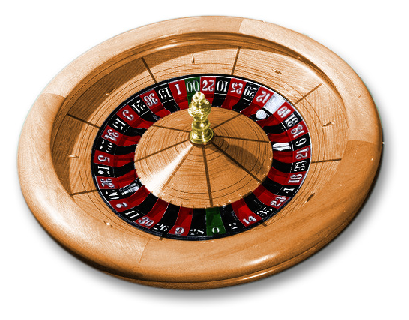 Figure 1: The wheel
Players arrive at the roulette table and offer the dealer money (either
cash or casino chips). In exchange, they are given special roulette
chips for betting at this wheel. These chips are not valid anywhere
else in the casino, and each player at the table has a unique color of
chips. Players bet by placing chips on a numbered layout, the wheel is
spun and a small white ball rolled around its edge. The ball lands on
a particular number in the wheel, which is the winning number for that
round, and is announced publicly by the dealer. Next, the dealer
clears away all losing bets, players who had bet on the winning number
(in some configuration) are paid in their own-colored chips and a new
round of betting begins.
Figure 2 shows a typical layout, along with the types of bets that can
be made. Unlike the wheel, the layout is arranged in numerical order.
Players can place their bets on varying places on the layout. Bets of
the type on the number 30 are called "straight up" bets. These are
bets on a single number. If the number comes up on the wheel, this bet
would pay the player 36 for 1 (35 to 1). That is, when 1 chip is bet,
the dealer pays the player 35 chips directly, and the chip that was bet
is not removed from the table. Bets of the type between the 8 and 11,
"line bets" are bets on two numbers. If either of the numbers comes
up, this bet pays the player 18 for 1. Players can also bet on
combinations of 3 numbers (by the 13) which pay 12 for 1, combinations
of 4 numbers (on the corner of 17-18-20-21) which pay 9 for 1, or
combinations of 6 numbers (by the 22-25) which pay 6 for 1. Players
can, of course, bet on "outside" bets like red/black, even/odd and
low/high. These bets will not be included in our analysis, as they are
not bet often enough to allow identification at the individual level,
but are discussed in our companion paper on aggregate behavior, Croson
and Sundali (2005).
Figure 1: The wheel
Players arrive at the roulette table and offer the dealer money (either
cash or casino chips). In exchange, they are given special roulette
chips for betting at this wheel. These chips are not valid anywhere
else in the casino, and each player at the table has a unique color of
chips. Players bet by placing chips on a numbered layout, the wheel is
spun and a small white ball rolled around its edge. The ball lands on
a particular number in the wheel, which is the winning number for that
round, and is announced publicly by the dealer. Next, the dealer
clears away all losing bets, players who had bet on the winning number
(in some configuration) are paid in their own-colored chips and a new
round of betting begins.
Figure 2 shows a typical layout, along with the types of bets that can
be made. Unlike the wheel, the layout is arranged in numerical order.
Players can place their bets on varying places on the layout. Bets of
the type on the number 30 are called "straight up" bets. These are
bets on a single number. If the number comes up on the wheel, this bet
would pay the player 36 for 1 (35 to 1). That is, when 1 chip is bet,
the dealer pays the player 35 chips directly, and the chip that was bet
is not removed from the table. Bets of the type between the 8 and 11,
"line bets" are bets on two numbers. If either of the numbers comes
up, this bet pays the player 18 for 1. Players can also bet on
combinations of 3 numbers (by the 13) which pay 12 for 1, combinations
of 4 numbers (on the corner of 17-18-20-21) which pay 9 for 1, or
combinations of 6 numbers (by the 22-25) which pay 6 for 1. Players
can, of course, bet on "outside" bets like red/black, even/odd and
low/high. These bets will not be included in our analysis, as they are
not bet often enough to allow identification at the individual level,
but are discussed in our companion paper on aggregate behavior, Croson
and Sundali (2005).
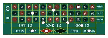 Figure 2: The layout
Notice that all these bets have the same expected value, -5.26%
on a double-zero wheel.8
Since the house advantage on (almost) all bets at the wheel is
the same, there is no economic reason to bet one way or another
(or for that matter, at all). In this paper, we will compare
actual betting behavior we observe against a benchmark of random
betting and search for systematic and significant deviations from
that benchmark.
Figure 2: The layout
Notice that all these bets have the same expected value, -5.26%
on a double-zero wheel.8
Since the house advantage on (almost) all bets at the wheel is
the same, there is no economic reason to bet one way or another
(or for that matter, at all). In this paper, we will compare
actual betting behavior we observe against a benchmark of random
betting and search for systematic and significant deviations from
that benchmark.
2 Method
The data were gathered from a large casino in Reno, Nevada, and
were also used in Croson and Sundali (2005) to examine aggregate
behavior.9 Casino executives supplied the
researchers with security videotapes for 18 hours of play of a
single roulette table. The videotapes consisted of three
separate six-hour time blocks over a 3-day period in July of
1998.10 The videotapes
provided an overhead view of the roulette area. The camera angle
was focused on the roulette layout to allow the coding of bets
placed and to protect player anonymity. Players were not
directly visible, however individual bets could be tracked by the
color of the chips being used. The videotape was subtitled with
a time counter. Note that while many casinos employ electronic
displays showing previous outcomes of the wheel, this casino had
no such displays at the time the data was collected.
A research assistant was employed to view and record player bet data
from these videotapes. Players were identified based upon the color of
the chips being used to bet, the player's location at the table, and
any distinct characteristics of the player's hand or arm such as
jewelry, clothing, tattoos, etc. Players who ran out of chips and
immediately bought more (of the same color) were coded as the same
player. Players who ran out of chips and did not immediately buy more
were coded as having left the table. When money was again exchanged
for chips of that particular color, we assumed a new player had joined
the table.11
The videotape methodology made it possible to view all of bets
made by each player with a high degree of accuracy. However,
while we could observe if a player bet on a particular
number, given the angle of the camera (from above), we could not
observe how many chips he or she bet on a particular
number. Thus we simplified the data recording to include simply
a bet being placed, without mention of how much the bet was. In
order to be consistent in not recording the amount bet, we coded
bets on multiple numbers (fractional bets like those in Figure 2)
the same as we recorded bets on single numbers. For example, a
player could place a single "corner bet" on 17, 18, 20, 21 by
placing his chip at the intersection of these numbers. We
recorded this bet as a bet placed on each of the four numbers.
We limit our analysis in this paper to bets placed in the inside
of the roulette layout, thus we do not count bets placed on
black/red, even/odd, high/low, 1,
2 or 3 12 or columns in
our data; the interested reader can find analysis of these
outside bets in aggregate in Croson and Sundali (2005). After
the assistant recorded all of the bets from the 18 hours of
videotape, one of the principal investigators performed an audit
check to insure accuracy.
3 Results
3.1 Descriptive Statistics: The Wheel and The Bets
Nine hundred and four spins of the roulette wheel were captured in this
data set (approximately 1 spin per minute). The expected frequency of
a single number on a perfectly fair roulette wheel is 1/38 or 2.6%. In
this sample the most frequent outcome was number 30 at 3.7%, the least
frequent outcome was number 26 at 1.7%. These data provide no evidence
that the wheel is biased.12 Table 1 presents the outcomes and the bets placed during
our sample.
Table 1: Spin outcomes and player bets
| | Frequency | Percent | Percent | Outcome - | Frequency | Percent |
| Outcome | outcome | outcome | expected | Expected | bet | bet |
|
0/0 | 22 | 0.024 | 0.026 | -0.002 | 354 | 0.016 |
| 0 | 25 | 0.028 | 0.026 | 0.001 | 442 | 0.020 |
| 1 | 23 | 0.025 | 0.026 | -0.001 | 362 | 0.016 |
| 2 | 30 | 0.033 | 0.026 | 0.007 | 450 | 0.020 |
| 3 | 28 | 0.031 | 0.026 | 0.005 | 357 | 0.016 |
| 4 | 15 | 0.017 | 0.026 | -0.010 | 375 | 0.017 |
| 5 | 28 | 0.031 | 0.026 | 0.005 | 636 | 0.028 |
| 6 | 20 | 0.022 | 0.026 | -0.004 | 363 | 0.016 |
| 7 | 15 | 0.017 | 0.026 | -0.010 | 682 | 0.030 |
| 8 | 26 | 0.029 | 0.026 | 0.002 | 633 | 0.028 |
| 9 | 23 | 0.025 | 0.026 | -0.001 | 503 | 0.022 |
| 10 | 24 | 0.027 | 0.026 | 0.000 | 484 | 0.021 |
| 11 | 26 | 0.029 | 0.026 | 0.002 | 783 | 0.035 |
| 12 | 21 | 0.023 | 0.026 | -0.003 | 360 | 0.016 |
| 13 | 21 | 0.023 | 0.026 | -0.003 | 525 | 0.023 |
| 14 | 27 | 0.030 | 0.026 | 0.004 | 649 | 0.029 |
| 15 | 27 | 0.030 | 0.026 | 0.004 | 340 | 0.015 |
| 16 | 25 | 0.028 | 0.026 | 0.001 | 643 | 0.029 |
| 17 | 23 | 0.025 | 0.026 | -0.001 | 1079 | 0.048 |
| 18 | 23 | 0.025 | 0.026 | -0.001 | 518 | 0.023 |
| 19 | 30 | 0.033 | 0.026 | 0.007 | 595 | 0.026 |
| 20 | 24 | 0.027 | 0.026 | 0.000 | 983 | 0.044 |
| 21 | 26 | 0.029 | 0.026 | 0.002 | 447 | 0.020 |
| 22 | 32 | 0.035 | 0.026 | 0.009 | 576 | 0.026 |
| 23 | 24 | 0.027 | 0.026 | 0.000 | 746 | 0.033 |
| 24 | 18 | 0.020 | 0.026 | -0.006 | 461 | 0.020 |
| 25 | 19 | 0.021 | 0.026 | -0.005 | 521 | 0.023 |
| 26 | 15 | 0.017 | 0.026 | -0.010 | 703 | 0.031 |
| 27 | 22 | 0.024 | 0.026 | -0.002 | 490 | 0.022 |
| 28 | 25 | 0.028 | 0.026 | 0.001 | 827 | 0.037 |
| 29 | 23 | 0.025 | 0.026 | -0.001 | 878 | 0.039 |
| 30 | 33 | 0.037 | 0.026 | 0.010 | 695 | 0.031 |
| 31 | 22 | 0.024 | 0.026 | -0.002 | 664 | 0.029 |
| 32 | 29 | 0.032 | 0.026 | 0.006 | 925 | 0.041 |
| 33 | 17 | 0.019 | 0.026 | -0.008 | 613 | 0.027 |
| 34 | 29 | 0.032 | 0.026 | 0.006 | 597 | 0.027 |
| 35 | 22 | 0.024 | 0.026 | -0.002 | 627 | 0.028 |
| 36 | 22 | 0.024 | 0.026 | -0.002 | 641 | 0.028 |
|
|
If players bet randomly, we would expect them to bet on each
number equally, thus 2.6% of the bets should fall on each
number, independently of the history of numbers which have
appeared. This independence is what we will test in our
analyses.
3.2 Gambler's fallacy vs. hot outcome
We will use a general linear model to analyze the probability of a bet
being placed on a number that has previously appeared, versus one which
has not. Our dependent variable,
Pit is binary; if a bet was placed on number i on spin t, we record a
success (1). If no bet was so placed, we record a failure (0). Thus
we will try to predict, on the basis of previous outcomes, whether a
player will bet on a particular number.
Independent variables include an intercept, a measure of the hotness of
a number, a control for the player's "favorite" numbers and a control
for leaving a bet on the table. We measure a number's hotness by
calculating a measure of how often the number i has appeared while the
player was at the table in the spins before spin t. In
particular, Hit is how many times number i has appeared
while the player was at the table before round t minus the expected
frequency of the number i appearing. This expected frequency is simply
(1-(37/38)) where (t-1) is the number of trials
observed by the player so far. This hotness measure thus calculates
the actual frequency of a number appearing minus the expected
frequency. If a number has appeared more than expected, this hotness
measure is positive, otherwise it is negative.
If players bet according to the gambler's fallacy, the probability of
their betting on a given number should be negatively related to its
hotness measure; numbers which have come up more frequently while they
were at the table are less likely to be bet on. In contrast, if
players bet according to the hot outcome, the probability of their
betting on a given number should be positively related to its hotness
measure. Notice that this hotness measure is calculated separately for
each individual in each period, based on what they have observed up to
the point of placing their bets.
Table 2: Hot outcome results by individual
| | 112 possible | 39 logistic models | 112 possible | 93 linear models |
| Coefficient | logistic models | w/o errors | linear models | w/o errors |
|
Negative Significant (GF) | 17 | 9 | 19 | 19 |
| Negative Nonsignificant (GF) | 39 | 11 | 36 | 29 |
| Positive Nonsignificant (HO) | 37 | 10 | 34 | 25 |
| Positive Significant (HO) | 19 | 9 | 23 | 20 |
|
|
The second independent variable is an attempt to control for the
baseline bets of individuals. Roulette players often bet the same
numbers consistently and repeatedly; the bets don't vary with past
outcomes. Thus, we need to control for these bets. Some players get
lucky and hit those numbers (and others don't), which could cause the
first type of players to look as though they were betting numbers which
had come up before and the second, those which hadn't. Instead, we
want to look at deviations from betting patterns as numbers
come up. Thus in the model, we include Fit, the
percentage of spins on which the player has bet on number i previously
to period t.
We expect the coefficient on this variable to be significant and
positive (if players bet on a number previously, they are more likely
to bet on it again). However, our main reason for including it is to
control for underlying personal preferences over numbers that might
bias our coefficient of interest, the hotness measure. Thus a
significant coefficient on the hotness measure measures a deviation
from the expected betting pattern of an individual, given their bets up
until now.
The final independent variable, Lit, controls for
a behavioral anomaly particular to roulette. When a bet wins, the
dealer pays the winnings directly to the player, but leaves the
winning chip on the same spot on the table. Many players are
reluctant to move this winning chip, claiming it is unlucky. If
we were to count that unmoved chip as a bet, we would bias the
results toward hot outcome, as players are often betting (by
default) on numbers that have won in the previous
round.13 We control for this behavior by including
an independent variable that equals one if an individual has bet
on a number in the previous round and it has won, and a zero
otherwise.
Thus our final model is
|
Pit = a0 + a1 Hit + a2 Fit +a3 Lit + e |
|
For each gambler we run two GLMs (one logistic and one linear). Of the
139 gamblers in our sample, not all had placed enough bets to allow us
to estimate these models either with or without errors. Table 2
categorizes the results of the coefficient on the hotness measure
(a1) for each individual using a variety of
techniques and error thresholds. Significant coefficients here
represent estimates that are significant at the 5% level using a
two-tailed test.
As Table 2 shows, we observe significant heterogeneity in the
population. Approximately half of the players in our data (depending
which model the reader prefers) can be categorized as gambler's fallacy
players; when a number has previously appeared, the probability of
their betting on it decreases. The other half of the players in our
data can be categorized as hot outcome players; when a number has
previously appeared, the probability of their betting on it increases.
One concern with this analysis, raised by an astute referee, is
that running so many regressions must result in some false
positives (or false negatives). To test for whether simple
chance is causing our results, we conducted two further analyses.
First, we looked at the underlying p-values from the regressions
in each column. If these values had been generated randomly, we
would expect them to be uniformly distributed between 0 and 1.
We compared the actual p-values to the uniform distribution using
the Kolgoromov-Smirnov test. We confidently reject the null
hypothesis that the p-values were generated by chance for each of
the four columns in Table 2 (p < .01 for all four comparisons).
Within each column, we run a similar test for the positive
significant/nonsignificant individuals, and the negative
significant/nonsignificant individuals. Again, we confidently
reject the null hypothesis that the p-values were generated by
chance for each (p < .01 for all eight comparisons).
A more discrete analysis examines the existing categorizations. If the
results were due to chance, we would expect 5% of the observations to
fall in the negative significant category, 45% in the negative
nonsignificant category, 45% in the positive nonsignificant category
and 5% in the positive significant category. We compare the actual
observations with this expected distribution using a chi-squared test.
We robustly reject the null that the p-values were observed by chance
(p < .0001 for all four columns). A similar test on only the
positive (negative) observations yields similar results
(p < .0001 for all eight comparisons).
Results from this field study are consistent with previous lab studies
demonstrating individual heterogeneity in gambler's fallacy/hot outcome
beliefs. While some gamblers cannot be classified reliably; those that
can are roughly equally split between betting in a fashion consistent
with the gambler's fallacy and the hot outcome. In the next subsection
we continue our analysis of roulette data by examining the hot hand and
stock of luck biases.
3.3 Hot hand vs. stock of luck
There is an important conceptual difference between a belief in hot
outcomes (e.g., hot numbers) and the hot hand (e.g., a hot person).
Our second set of analyses investigates whether individual's behavior
is consistent with hot hand beliefs. To do this, we analyze whether
gamblers bet on more or fewer numbers in response to previous wins and
losses. Thus, if I've won in the past, I am hot and more likely to be
(more) in the future.
We first examine the average number of bets an individual places after
winning on the previous spin and after losing on the previous spin. If
the former is greater than the latter, we say this person bets
consistently with the hot hand. If the reverse, we say this person
bets consistently with stock of luck. Of our 139 gamblers, 62 bet
consistently with the hot hand and 32 with the stock of luck bias. Of
the remaining 45 gamblers, 31 of them either only won or only lost at
the table in our sample while 14 played for only one spin of the wheel.
As a second, more formal analysis we run a general linear model for each
individual. The dependent variable is the number of bets placed on spin
t and the independent variables include an indicator variable
describing whether the individual has won or lost on spin t-1. Table 3
reports the number of subjects whose parameter value falls into each
category. Ninety-six subjects could be categorized in this way without
errors.
As with the previous analysis of the gambler's fallacy versus the
hot outcome, we find significant individual heterogeneity in the
hot hand/stock of luck biases. Here, more subjects act
consistently with the hot hand bias (which predicts a positive
relationship between previous wins and number of bets placed)
than with the stock of luck bias (which predicts a negative
relationship). Similar reliability tests as those described
above yield similar results (p < .01 for the
Kolgoromov-Smirnov tests and p < .001 for the chi-squared
tests).
Table 3: Hot hand results by individual
| | 96 linear models |
| Coefficient | without errors |
|
Negative Significant (SL) | 6 |
| Negative Nonsignificant (SL) | 37 |
| Positive Nonsignificant (HH) | 41 |
| Positive Significant (HH) | 12 |
|
|
3.4 Correlation of Biases
Our data allow us to independently characterize individuals as gambler's
fallacy/hot outcome players and as hot hand/stock of luck players. A
further analysis examines the distribution of players over those four
types. Table 4 presents this distribution, categorizing players based
on the general linear models at the individual level reported in Table
2 (the final column) and Table 3 including those categorized as
directional.14 We
exclude 11 players who are categorized on one dimension and not on
another.
Table 4: Relationship between the biases
| | Hot outcome | Gambler's fallacy |
|
Hot Hand | 10 | 42 |
| Stock-of-Luck | 32 | 5 |
|
|
A chi-squared test strongly rejects the null hypothesis of no
relationship between the biases (p < .0001). In particular,
there appears to be a correlation; players who act consistently with
the gambler's fallacy (betting on numbers that haven't appeared
previously), are more likely to act consistently with the hot hand
(increasing the number of bets they place after a win). Almost half
the subjects are in this first category, consistent with previous
research demonstrating both biases in the lab. In contrast, players
who act consistently with the hot outcome (betting on numbers that have
appeared previously), are more likely to act consistently with the
stock-of-luck bias (decreasing the number of bets they place after a
win).
This relationship can be seen in Figure 3, below. Here we graph, for
each of the 89 individuals characterized in Table 5, their regression
parameters on the two biases.
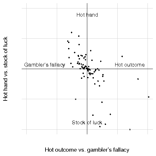 Figure 3: Relationship between biases
What accounts for the pattern of individual beliefs found in
Figure 3? While further research will be necessary to flesh out
the variables underlying these patterns, we propose locus of
control as an organizing explanation for this pattern.
Originally developed by Rotter (1964), Zimbardo (1985) defines
locus of control as: "... a belief about whether the outcomes
of our actions are contingent on what we do (internal locus of
control) or on events outside our personal control (external
control orientation)" (p. 275).
Generally a person with an internal locus of control attributes outcomes
to personal decisions and efforts while a person with an external locus
of control attributes outcomes to chance or other external factors.
Applying this concept to roulette, a person with an internal locus of
control is likely to attribute previous wins to the decisions he made
and thus to connect such winning with gambling skill. If a player has
just won because of skill, then these skills should lead to more
winning, which explains why players with such beliefs increase their
bets after winning, exhibiting hot hand behavior. On the other hand, a
person with an external locus of control attributes winning to simply
luck. Thus a person with external locus of control concludes that
winning again after a previous win is less likely and will decrease
their bets after winning, exhibiting stock of luck behavior.
Remember that while the hot hand/stock of luck describes beliefs of
outcomes of the individual (like wins and losses), the gambler's
fallacy/hot outcome describes beliefs about outcomes of the random
process (like heads or tails). So how would the beliefs of a person
with an internal or external locus of control differ regarding random
processes?
Consider first the person who has an external locus of control
and thus attributes outcomes to luck (stock of luck). If one
believes luck is in control of a random process and three heads
in a row have appeared, then one should believe that luck will
continue to control the outcomes and that another head will
appear. Put another way, players who believe in luck are more
likely to believe in streaks (hot outcomes) because luck produces
streaks. Thus the external locus of control causes both stock of
luck and hot outcome beliefs.
In contrast, a person with an internal locus of control who believes
that winning is a result of skill is likely to reject the idea that the
process producing the outcomes is random since this would mitigate the
skill involved. A more plausible belief is that outcomes on the
roulette wheel are controlled by some process that can be learned or
discerned by the use of skill. When the internal person wins, it is
confirmation that she has ascertained the pattern and this confidence
leads her to bet more on the next spin of the wheel (hot hand). The
most plausible cognitive explanation for her supposed pattern-detecting
skill is representativeness, which explains why she bets consistently
with the gambler's fallacy. Thus the internal locus of control causes
both hot hand and gambler's fallacy beliefs.
Unfortunately we could not collect locus of control or other personality
measures from our casino patrons, and thus cannot test our speculation
of the underlying causes of the relationship between these two biases.
Further lab testing will be necessary to address this question, and to
compare this speculation with other candidate explanations for our
results.
Figure 3: Relationship between biases
What accounts for the pattern of individual beliefs found in
Figure 3? While further research will be necessary to flesh out
the variables underlying these patterns, we propose locus of
control as an organizing explanation for this pattern.
Originally developed by Rotter (1964), Zimbardo (1985) defines
locus of control as: "... a belief about whether the outcomes
of our actions are contingent on what we do (internal locus of
control) or on events outside our personal control (external
control orientation)" (p. 275).
Generally a person with an internal locus of control attributes outcomes
to personal decisions and efforts while a person with an external locus
of control attributes outcomes to chance or other external factors.
Applying this concept to roulette, a person with an internal locus of
control is likely to attribute previous wins to the decisions he made
and thus to connect such winning with gambling skill. If a player has
just won because of skill, then these skills should lead to more
winning, which explains why players with such beliefs increase their
bets after winning, exhibiting hot hand behavior. On the other hand, a
person with an external locus of control attributes winning to simply
luck. Thus a person with external locus of control concludes that
winning again after a previous win is less likely and will decrease
their bets after winning, exhibiting stock of luck behavior.
Remember that while the hot hand/stock of luck describes beliefs of
outcomes of the individual (like wins and losses), the gambler's
fallacy/hot outcome describes beliefs about outcomes of the random
process (like heads or tails). So how would the beliefs of a person
with an internal or external locus of control differ regarding random
processes?
Consider first the person who has an external locus of control
and thus attributes outcomes to luck (stock of luck). If one
believes luck is in control of a random process and three heads
in a row have appeared, then one should believe that luck will
continue to control the outcomes and that another head will
appear. Put another way, players who believe in luck are more
likely to believe in streaks (hot outcomes) because luck produces
streaks. Thus the external locus of control causes both stock of
luck and hot outcome beliefs.
In contrast, a person with an internal locus of control who believes
that winning is a result of skill is likely to reject the idea that the
process producing the outcomes is random since this would mitigate the
skill involved. A more plausible belief is that outcomes on the
roulette wheel are controlled by some process that can be learned or
discerned by the use of skill. When the internal person wins, it is
confirmation that she has ascertained the pattern and this confidence
leads her to bet more on the next spin of the wheel (hot hand). The
most plausible cognitive explanation for her supposed pattern-detecting
skill is representativeness, which explains why she bets consistently
with the gambler's fallacy. Thus the internal locus of control causes
both hot hand and gambler's fallacy beliefs.
Unfortunately we could not collect locus of control or other personality
measures from our casino patrons, and thus cannot test our speculation
of the underlying causes of the relationship between these two biases.
Further lab testing will be necessary to address this question, and to
compare this speculation with other candidate explanations for our
results.
4 Conclusions and discussion
This paper uses observational data to demonstrate the existence and
impact of the hot hand and gambler's fallacy biases. We demonstrate
the existence of significant biases even in this, sophisticated,
population, providing an important robustness check on previous
laboratory data. Like this previous research, we observe significant
individual heterogeneity in the population. Our participants are split
almost evenly between betting in a way consistent with the gambler's
fallacy and consistent with the hot outcome.
Importantly, however, our data allow us to investigate the
correlation of these biases at the individual level. We find
that gambler's fallacy players are more likely to also be hot
hand gamblers. These relationships suggest there may be an
underlying construct determining biased beliefs that further
research might illuminate. Candidates for this construct have
been suggested by us and others (locus of control,
representativeness, cognitive reflection of Frederick [2005]),
but further research in the lab will be need to identify these
potential mediators.
These results are consistent with those previously observed in
the lab (e.g., Ayton & Fischer, 2004; Chau & Phillips, 1995).
That these observations are robust in the field with real money
on the line and real participants is reassuring. However, the
limitations inherent in field data admit of alternative
interpretations of our results. For example, the hot outcome
effect may be explained by an availability bias; individuals are
more likely to bet on numbers that have recently won not because
they believe these numbers more likely to win again but instead
because they're easily called to mind. The hot hand effect may
be explained by an income or house money effect; individuals bet
on more numbers after they have won not because they believe that
they (personally) are more likely to win again but because
they're richer, or are playing with the house's money. While
these alternative explanations can explain some results, they
don't provide satisfactory explanations for the heterogeneity of
the data at the individual level, nor for the correlation between
the biases observed within the individual.
These limitations suggest further research combining empirical
and questionnaire data in a way that we were prevented from
accomplishing here. For example, a think-aloud protocol might
provide evidence in favor or against these alternative
explanations. Gathering psychological measures like locus of
control as well as demographic information might help us to
predict what type of biased beliefs an individual is likely to
have. Finally, our data infers beliefs from observed actions;
eliciting beliefs directly via a questionnaire, then observing
actions would provide a useful check on our results. These
combinations of field and lab data are attractive, but will
require extreme cooperation from a casino, which is not currently
available.
Other future projects might involve data from other non-autocorrelated
casino games (e.g., craps, slot machines) both to replicate our current
findings and to search for differences between the games. Finally,
there are a number of other questions one might explore using the
existing data including conformity (the correlation of betting across
players as in Blank, 1968), the status quo bias (probability of leaving
winning bets as they lie), the psychology of near misses (when an
individual's bet almost wins), and when players leave the game
(breaking even, busting out). While these data are not as targeted as
that from the lab, we see empirical data as an opportunity to provide a
robustness-check on (and external validity for) experimentally-observed
biases.
Almost every decision we make involves uncertainty in some way, both
over individual events and over sequences of events. Previous research
has demonstrated a number of biases in how individuals perceive and
react to this uncertainty, but the demonstrations have been primarily
in the lab, using undergraduate student participants. This paper uses
data from individuals gambling with their own money in a casino to test
for the presence of these biases in a naturally-occurring environment.
The behavior we observe is indeed consistent with previously-observed
biases, providing an important robustness check on the previous
research. We observe significant individual heterogeneity among the
population in their direction and strength of each bias.
In addition, our data allows us to identify these biases separately
within each individual, and to examine the correlation between them.
We find a significant and positive correlation between individuals who
act in accordance with gambler's fallacy beliefs and with hot hand
beliefs, suggesting a unifying cause for the two illusions. Further
research will be needed to identify this cause, and to help us predict
an individual's biases and their resulting actions.
References
Ayton, P. & Fischer. I. (2004). The gambler's fallacy and the
hot-hand fallacy: Two faces of subjective randomness? Memory
and Cognition, 32, 1369-1378.
Baron, J. & Ritov, I. (2004). Omission bias, individual differences,
and normality. Organizational Behavior and Human Decision
Processes, 94, 74-85.
Blais, A-R., & Weber, E. U. (2006). A domain-specific
risk-taking (DOSPERT) scale for adult populations.
Judgment and Decision Making, 1, XX-XX.
Blank, A. D. (1968). Effects of group and individual conditions
on choice behavior. Journal of Personality and Social
Psychology, 8, 294-298.
Chau, A. & Phillips, J. (1995). Effects of Perceived Control Upon
Wagering and Attributions in Computer Blackjack. The Journal
of General Psychology, 122, 253-269.
Croson, R. & Sundali, J. (2005). The gambler's fallacy and the hot
hand: Empirical data from casinos. Journal of Risk and
Uncertainty, 30, 195-209.
Edwards, W. (1961). Probability learning in 1000 trials.
Journal of Experimental Psychology, 62, 385-394.
Estes, W. K. (1964). Probability learning. In A. W. Melton (ed.),
Categories of Human Learning. New York: Academic Press.
Ethier, S. N. (1982). Testing for favorable numbers on a roulette
wheel. Journal of the American Statistical Association, 77,
660-665.
Feldman, J. (1959). On the negative recency hypothesis in the
prediction of a series of binary symbols. American Journal of
Psychology, 72, 597-599.
Friedland, N. (1998). Games of luck and games of chance: The effect
of luck- versus chance-orientation on gambling decisions.
Journal of Behavioral Decision Making, 11, 161-179.
Frederick, S. (2005). Cognitive reflection and decision making.
Journal of Economic Perspectives, 19, 25-42.
Gal, I. & Baron. J. (1996). Understanding repeated choices.
Thinking and Reasoning, 2, 81-98.
Gilovich, T., Vallone, R. & Tversky, A. (1985). The hot hand in
basketball: On the misperception of random sequences.
Cognitive Psychology, 17, 295-314.
Harris, C. R., Jenkins, M., & Glaser, D. (2006). Gender
differences in risk assessment: Why do women take fewer risks
than men? Judgment and Decision Making, 1, XX-XX.
Kahneman, D. & Tversky, A. (1972). Subjective probability: A
judgment of representativeness. Cognitive Psychology, 3,
430-454.
Keren, G. & Lewis, C. (1994). The two fallacies of gamblers: Type I
and Type II. Organizational Behavior and Human Decision
Processes, 60, 75-89.
Keren, G. & Wagenaar, W.. (1985). On the Psychology of Playing
Blackjack: Normative and Descriptive Considerations with Implications
for Decision Theory. Journal of Experimental Psychology:
General, 114, 133-158.
Langer, E. (1975). The illusion of control. Journal of
Personality and Social Psychology, 32, 311-328.
Lee, W. (1971). Decision theory and human behavior. New
York: Wiley.
Leopard, A. (1978). Risk preference in consecutive gambling.
Journal of Experimental Psychology: Human Perception and
Performance, 4, 521-528.
Lindman, H., & Edwards, W. (1961). Supplementary report: Unlearning
the gambler's fallacy. Journal of Experimental Psychology,
62, 630.
Oldman, D. (1974). Chance and skill: A study of roulette.
Sociology, 8, 407-426.
Rapoport, A. & Budesceu, D. (1992). Generation of random series in
two-person strictly competitive games. Journal of Experimental
Psychology: General, 121, 352-363.
Ritov, I. & Baron, J. (1992). Status-quo and omission bias.
Journal of Risk and Uncertainty, 5, 49-61.
Rotter, J. B. (1966). Generalized expectancies for internal vs. external
control of reinforcement. Psychological Monographs, 80, 1-28.
Samuelson, W. & Zeckhauser, R. (1988). Status quo bias in decision
making. Journal of Risk and Uncertainty, 1, 7-59.
Thaler, R. H., & Johnson, E. J. (1990). Gambling with the house
money and trying to break even: The effects of prior outcomes on
risky choice, Management Science 36, 643-660.
Tversky, A. & Kahneman, D. (1971). Belief in the law of small
numbers. Psychological Bulletin, 76, 105-110.
Tversky, A. & Kahneman, D. (1974). Judgement under uncertainty:
Heuristics and biases. Science, 185, 1124-1131.
Wagenaar, W. (1972). Generation of random sequences by human subjects:
A critical survey of literature. Psychological Bulletin, 77,
65-72.
Wagenaar, W. (1988). Paradoxes of gambling behavior. Lawrence
Erlbaum Associates, London, UK.
Weber, E. U., Anderson, C. J. & Birnbaum, M. H. (1992). A
theory of perceived risk and attractiveness.
Organizational Behavior and Human Decision Processes,
52, 492-523.
Zimbardo, P. G. (1985). Psychology and Life. Glenview,
IL: Scott Foreman and Company.
Footnotes:
1The authors thank Eric Gold for
substantial contributions in earlier stages of this research.
Thanks also to Jeremy Bagai, Dr. Klaus von Colorist, Bradley
Ruffle, Paul Slovic, Willem Wagenaar, participants of the
J/DM and ESA conferences, at the Conference on Gambling and
Risk Taking and at seminars at Wharton, Caltech and INSEAD
for their comments on this paper. Special thanks to the
Institute for the Study of Gambling and Commercial Gaming for
industry contacts which resulted in the acquisition of the
observational data reported here. Financial support from NSF
SES 98-76079-001 is also gratefully acknowledged. All
remaining errors are ours. Address correspondence to Rachel
Croson, 567 JMHH, The Wharton School University of
Pennsylvania, 3730 Walnut Street, Philadelphia, PA
19104-6340,
crosonr@wharton.upenn.edu.
James Sundali's email is
jsundali@unr.nevada.edu
2Or, more generally, a belief in a more
negative autocorrelation than is present. Thus when an
individual overestimates the amount of negative autocorrelation
in any sequence, we could say they were exhibiting gambler's
fallacy beliefs as well.
3Or, more generally, a belief in a more
positive autocorrelation than is present. Thus when an
individual overestimates the amount of positive autocorrelation
in any sequence, we could say they were exhibiting hot outcome
beliefs as well.
4The hot outcome bias is related but not identical
to the construct referred to by Keren and Lewis (1994) as the gambler's
fallacy type II. They present results of a questionnaire study in the
lab demonstrating that individuals underestimate the number of
observations necessary to detect biased roulette wheels. Thus after
seeing even a small streak of red numbers, gamblers might believe the
wheel is biased and expect more red numbers. The number of spins
participants believe they need to observe to detect a biased wheel,
while significantly smaller than the true number of spins necessary, as
derived in Ethier (1982), is significantly larger than the number of
spins any individual in our data set will observe.
5One can construct other explanations for the
behavior we here attribute to the hot outcome. For example,
perhaps numbers that have recently hit on the roulette wheel
are more available to the gambler than other numbers.
This availability may cause the gambler to bet on numbers that
have recently hit. Unfortunately in our empirical data we will
not be able to distinguish between these alternative causes of
this behavior, although previous lab research can and has done
so.
6As with the hot outcome above,
there are alternative explanations for these behaviors as well.
For example, wealth effects or house money effects might cause
an increase in betting after a win (hot hand) (Thaler &
Johnson 1990). Prospect theory's assumption of increased
risk-seeking in losses might cause an increase in betting after
a loss (stock of luck). In the lab, these effects can be
separated by eliciting beliefs directly as in Ayton and Fischer
(2004). In our empirical data we will not be able to
distinguish between these alternative explanations.
7Our companion paper, Croson and
Sundali (2005) has examined thee data at the aggregate level. There we
provide evidence that the wheel is unbiased, that gambler's fallacy
behavior is observed in outside bets after long streaks (5 and 6
observations of the same type), and that, in aggregate, individuals
place more bets after they have won a previous bet than after they have
lost one (or than on their first spin).
8This statement is not strictly
true. One bet has a house advantage of 7.89%. The bet
involves placing a chip on the outside corner of the layout
between 0 and 1. The bet wins if 0, 00, 1, 2 or 3 appears, but
pays only 6 for 1 (as though the bet were covering 6 numbers
instead of 5). We observed only 75 instances of this bet being
placed (out of 22,527 bets). Only 11 different individuals
placed this bet (out of 139 identifiable individuals in our
data), and of them, only 6 placed this bet more than twice.
9At the time of data collection a casino in
Washoe County, Nevada, was classified as "large" by the Nevada
Gaming Control Board if total (yearly) gaming revenues for the
property exceeds $36 million.
10The three time blocks were from 4:00 p.m. to 10:00
p.m., 8:00 p.m. to 2:00 a.m., and 10:00 p.m. to 4:00 a.m.
These time blocks were appropriate since the majority of gaming
business is done in the evening hours.
11This coding has the potential to introduce two
possible errors; two different people could be counted as the same
person, or the same person could be counted as two different people.
We believe that the first of these errors is minimized; when chips were
depleted and someone immediately purchased more, the coder could
recognize from their hand characteristics if it was the same person.
Additionally, this casino has many roulette tables, it was rare that
this table was full or that people were waiting to buy in immediately
after someone had gone bust. The second error may be somewhat more
likely, here we rely on the observation that if an individual wants to
rebuy, (s)he rarely waits to do so.
12 Based on the work of Ethier (1982),
Keren and Lewis (1994) report that the number of observations necessary
to detect a favorable number (bias) is generally quite large. For
example, on a wheel with 37 numbers it would be necessary to view
30,195 spins in order to detect a bias of 1/33 with a 90% level of
certainty.
13This behavior is consistent with the status quo
bias (Samuelson and Zeckhauser 1988) or the omission/commission
bias (Ritov and Baron 1992, Baron and Ritov 2004), as this chip
represents a bet that has been placed by default. Thus one can
interpret a positive significant coefficient on this variable
as evidence for these biases in this dataset. A positive
coefficient on this variable is also consistent with Wagenaar
(1988) who found 70 out of 75 winning bets in his data were not
moved. However, as this is not the main focus of our paper, we
do not provide a lengthy discussion of this finding.
Interested readers are encouraged to contact the author for
further discussion.
14Other possible categorizations yield
qualitatively identical results (e.g., using those categorized both
significantly and nonsignificantly regardless of error, restricting
attention to those categorized significantly, either only without error
or all and using the logistic models to categorize the Gambler's
Fallacy/Hot Outcome subjects rather than the linear models).
File translated from
TEX
by
TTH,
version 3.74.
On 17 Jul 2006, 04:07.