Decision analysis: a formal prescriptive method

Decisions that are "complex" in the effects they have
Attempts to do better than ordinary decision making, by the standards of utility maximization.
Two types: probabilities and multiattribute
These can be combined

Example of decision with probabilities:
amniocentesis

Here is an example for p(downs)=.00274. The example also assumes that the abortion rate is higher than this (.00371) becasue of false positive test results, but recent studies tend to assume a false-positive rate very near zero.

Calculation of relative EU of testing vs. not testing

The following form calculates the utility of testing vs. not testing using the formula:
disutlity of no test - disutility of test, or
p(down)*u(down) - [p(miscarry)*u(miscarry) + p(abort)*u(abort)]

Assuming that p(abort) is the same as p(down) (i.e., abortion if test is positive, no false positives), this becomes:
p(down)*u(down) - [p(miscarry)*u(miscarry) + p(down)*u(abort)], or
p(down)*u(down) - p(miscarry)*u(miscarry) - p(down)*u(abort), or
p(down)*[u(down) - u(abort)] - p(miscarry)*u(miscarry)

Amniocentesis calculator (for illustration only)

Figures are from here

Effects of age

risks as a function of age

From N. Sicherman and A. Ferber

Why we need multi-attribute utility theory (MAUT)

Dilbert cartoon

How to do MAUT

Decide what the important aspects of the decision are.
Collect your options.
Rank options on each dimension.
Assign end point utility weights to best and worst. Scale on this is arbitrary. We often use0 for the worst, 100 for the best.
Assign intermediate utilities for the rest.
- This can be done by direct judgment.
- This can also be done by any other method, such as standard gambles or time tradeoff.
- Usually this is monotonic. When not?
Assign weights to dimensions. Not all dimensions are equally important. MOST CRITICAL STEP.

Example: birth control

	HIV	STD	Hlth.	Preg.	Easy	Sex	TOTAL
	prev.	prev.	risk	prev.	use	pleas.	UTIL.
IUD	0	0	0	96	50	100	196.8
Pill	0	0	50	94	80	100	247.2
Norplant	0	0	0	99	100	100	219.2
Condom	99	99	90	84	0	90	377.7
Diaphr.	0	0	90	82	0	95	232.6
None	0	0	90	15	100	100	224.0
Abstain	100	100	100	100	100	0	350.0
WEIGHT	1.00	.50	.80	.80	.40	1.00

For condom, the sum is 1.00 ·99 + .50 ·99 + .80 ·90 + .80 ·84 + .40 ·0 + 1.00 ·90 = 377.7 .

Analysis of life (from Baron et al., 2001)

Pain, fatigue, and discomfort: 0 = no effect; 100 = as bad as death.
Economic standard of living: 0 = no effect; 100 = dire poverty.
Work: 0 = no effect; 100 = unable to do any work.
Love life: 0 = no effect; 100 = love life nonexistent.
Family life: 0 = no effect; 100 = family life nonexistent.
Spiritual life: 0 = no effect; 100 = spiritual life nonexistent.
Leisure activities: 0 = no effect; 100 = activities nonexistent.

Please try to interpret these descriptions so that they do not count the same effects twice. For example, if "spiritual life" includes communing with nature, do not also count this as part of "leisure".

Singer's analysis of life (roughly)

Experience

Ongoing plans, personhood

Attachments

(Desire for) potential

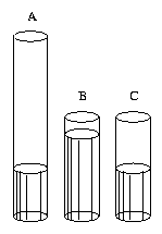
The idea of weight

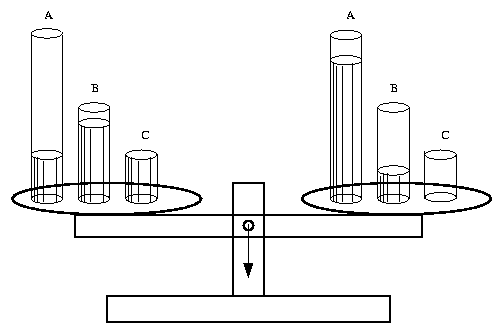
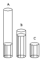
We can think of a decision as a balancing of two (or more) options. Each option here has 3 attributes. Each attribute is represented by a container that is full of a certian amount of its type of utility (utility-on-attribute). The utility-on-attribute numbers represent the percents full. The weights represent the sizes of the containers.

How weight depends on range

Attribute	A	B	C
Utility on attribute	25	80	100
Weight	1.00	0.55	0.275
Utility	25	44	27.5

The table shows the numbers and weights for the option on the left above. The weights are relative to the first attribute.

The utility-on-attribute numbers are relative to the top and bottom of each container. If the top goes up, then the utility number assigned to the same level must go down, but the weight of the attribute will go up. The weight thus depends on the range. The range is the difference between the top and bottom.

For example, change attribute C's range.

Attribute	A	B	C
Utility on attribute	25	80	100
Weight	1.00	0.55	0.275
Utility	25	44	27.5

Attribute	A	B	C
Utility on attribute	25	80	50
Weight	1.00	0.55	0.55
Utility	25	44	27.5

The reference point for the attribute utility has changed. As a result, the utility-on-attribute and the weight of C change, but the final utility is the same.

The most important point here is that we cannot compare weights without knowing the top and bottom of each range (container).

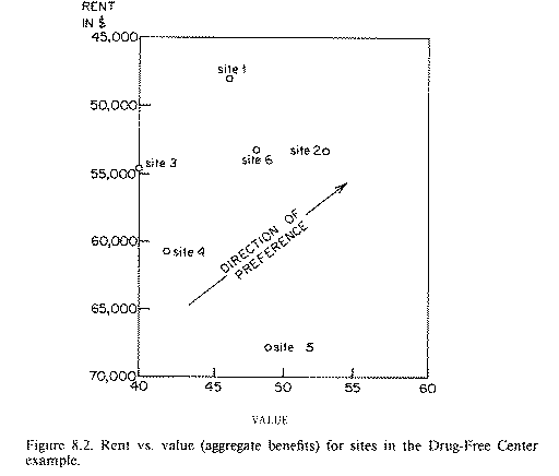
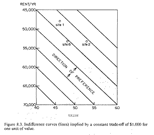
Indifference curves (Von Winterfeldt and Edwards)

Using one attribute to measure another

Consistency check: Thomson condition

The point is that a certain change in one attribute - from X to Y, or from Y to Z - has the same effect on utility, regardless of the level of the other attribute(s). If the change bumps you up to the next level (the next indifference curve), it will do this no matter which curve you start on.

Independence in 3D

A simpler test involves three dimensions. The idea of preferential independence is that the tradeoff of any two dimensions does not depend on the level of any others. If a change from X to Y is compensated by a change from 128 to 64 (as it is), that fact remains true regardless of the levels of other attributes.

The basic idea is that we can add utilities of attributes. This is a psychological condition. It is about what you value. It is not about correlations in the world. The space of possibilities shown in these graphs need not exist. It might be that only the two points labeled "T" exist, so that there is a perfect correlation between price and memory. It doesn't matter, because we can imagine the other points.

Example from Gardiner and Edwards

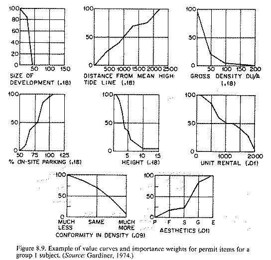
California coast (before)

California coast (after)

Effects of MAUT: Gardiner and Edwards

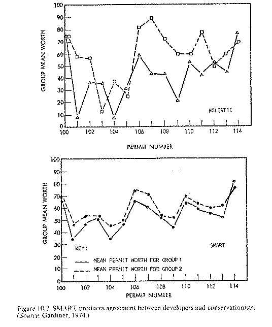
The main insight (Keeney)

5.4 Prioritizing Objectives

It is natural when thinking about objectives to think about their relative importance. In evaluating possible employment offers, you may naturally wish to maximize your salary and minimize your commuting time. Which of these objectives is more important? Suppose it is salary. Then is salary five times more important? As we will see below, it is not possible to answer such questions so that the response is unambiguous. When we quantify objectives by simply asking for their relative importance, considerable misinformation about values is produced and a substantial opportunity to understand values is lost.

The importance of an objective must depend on how much achievement of that objective we are talking about. Clearly a cost of $200 million is more important than a cost of $4 million. So if somebody asks whether the environmental risk at a hazardous waste site is more important than the cleanup cost, it should make a difference whether the cost is $4 million or $200 million. Let us examine this in more detail and then discuss how objectives should be prioritized.

The Most Common Critical Mistake

There is one mistake that is very commonly made in prioritizing objectives. Unfortunately, this mistake is sometimes the basis for poor decisionmaking. It is always a basis for poor information. As an illustration, consider an air pollution problem where the concerns are air pollution concentrations and the costs of regulating air pollution emissions. Administrators, regulators, and members of the public are asked questions such as "In this air pollution problem, which is more important, costs or pollutant concentrations?" Almost anyone will answer such a question. They will even answer when asked how much more important the stated "more important" objective is.

For instance, a respondent might state that pollutant concentrations are three times as important as costs. While the sentiment of this statement may make sense, it is completely useless for understanding values 148 or for building a model of values. Does it mean, for example, that lowering pollutant concentrations in a metropolitan area by one part per billion would be worth the cost of $2 billion? The likely answer is "of course not." Indeed, this answer would probably come from the respondent who had just stated that pollutant concentrations were three times as important as costs. When asked to clarify the apparent discrepancy, he or she would naturally state that the decrease in air pollution was very small, only one part in a billion, and the cost was a very large $2 billion. The point should now be clear. It is necessary to know how much the change in air pollution concentrations will be and how much the costs of regulation will be in order to logically discuss and quantify the relative importance of the two objectives.

This error is significant for two reasons. First, it doesn't really afford the in-depth appraisal of values that should be done in important decision situations. If we are talking about the effects on public health of pollutant concentrations and billion-dollar expenditures, I personally don't want some administrator to give two minutes of thought to the matter and state that pollutant concentrations are three times as important as costs. Second, such judgments are often elicited from the public, concerned groups, or legislators. Then decisionmakers use these indications of relative importance in inappropriate ways.

The Clean Air Act of the United States provides an illustrative example. This law essentially says that the health of the public is of paramount importance and that costs of achieving air pollutant levels should not be considered in setting standards for those levels. Of course, this is not practical or possible or desirable in the real world. After spending hundreds of billions of dollars, we could still improve our air quality further with additional expenditures. This would be the case even if we could only further improve the "national health" by reducing by five the annual number of asthma attacks in the country. If the value tradeoffs are done properly and address the question of how much of one specific attribute is worth how much of another specific attribute, the insights from the analysis are greatly increased and the likelihood of misuse of those judgments is greatly decreased.