Guessing means

-0.35 0.06 0.68 -1.90 0.98 0.73 0.96 -1.52 0.11 -0.55 0.42 0.75 0.87 -0.04 0.17 0.01 -0.53 0.77 0.17 0.31

0.26 -1.01 -1.47 0.57 0.55 -0.68 -0.46 -2.87 -0.19 -0.91 -0.89 -2.52 -1.95 0.33 -1.97 -0.97 -0.73 -0.44 -1.44 -0.40

-1.36 -2.69 -0.62 -1.01 0.89 -0.40 0.14 0.01 -0.63 -0.63 -0.36 1.04 0.53 -0.93 2.10 -1.02 -0.93 0.40 0.31 1.10

4.39 5.53 4.11 3.44 4.67 7.73 5.07 5.77 5.17 6.52 4.61 5.35 4.26 4.13 6.50 5.43 5.05 6.50 4.10 2.82

0.56 0.81 1.11 0.72 -1.04 0.53 0.57 1.38 0.09 0.99 0.18 2.67 0.59 1.52 0.63 1.88 1.38 0.86 0.58 1.68

3.29 2.57 3.37 1.78 1.83 2.42 2.28 3.12 1.02 1.66 1.87 3.73 2.10 2.61 1.62 0.25 2.99 1.49 2.23 3.31

-0.82 -0.16 -1.81 -2.58 -1.28 -2.69 -2.78 -1.40 -4.54 -2.35 -1.16 -2.74 -1.48 -1.90 -2.83 -3.82 -1.24 -2.26 -2.64 -1.46

Guessing means

-0.35 0.06 0.68 -1.90 0.98 0.73 0.96 -1.52 0.11 -0.55 0.42 0.75 0.87 -0.04 0.17 0.01 -0.53 0.77 0.17 0.31 (.10)

0.26 -1.01 -1.47 0.57 0.55 -0.68 -0.46 -2.87 -0.19 -0.91 -0.89 -2.52 -1.95 0.33 -1.97 -0.97 -0.73 -0.44 -1.44 -0.40 (-.86)

-1.36 -2.69 -0.62 -1.01 0.89 -0.40 0.14 0.01 -0.63 -0.63 -0.36 1.04 0.53 -0.93 2.10 -1.02 -0.93 0.40 0.31 1.10 (-.20)

4.39 5.53 4.11 3.44 4.67 7.73 5.07 5.77 5.17 6.52 4.61 5.35 4.26 4.13 6.50 5.43 5.05 6.50 4.10 2.82 (5.06)

0.56 0.81 1.11 0.72 -1.04 0.53 0.57 1.38 0.09 0.99 0.18 2.67 0.59 1.52 0.63 1.88 1.38 0.86 0.58 1.68 (.88)

3.29 2.57 3.37 1.78 1.83 2.42 2.28 3.12 1.02 1.66 1.87 3.73 2.10 2.61 1.62 0.25 2.99 1.49 2.23 3.31 (2.28)

-0.82 -0.16 -1.81 -2.58 -1.28 -2.69 -2.78 -1.40 -4.54 -2.35 -1.16 -2.74 -1.48 -1.90 -2.83 -3.82 -1.24 -2.26 -2.64 -1.46 (-2.10)

Example

m1	m2	f
B+	B+	87
B-	D+	67
B+	D+	69
D+	B-	75
A	B-	83
B-	C	73
C	D+	65
B+	C	75
C	B-	77

m1	m2	f
B+	B-	81
D+	B+	81
A	A	95
D+	D+	63
B-	B+	85
C	A	89
B-	A	91
D+	C	69
B+	A	93

On the basis of the students on the left, predict f for these:

	m1	m2	Prediction	Answer	Model
1.	C	C
2.	A	C
3.	B-	B-
4.	C	B+
5.	A	B+

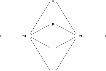
The model is the model of your judgments, MUD.

Example of calculation of correlation

                                    Mean  s.d.
Correct answers    71 77 79 83 89   79.8  6.72
Judge's answers    69 79 80 85 87   80    7.00
Model's answers    71 77 79 83 89 (decimals omitted)

The best model of the judge is f = 1.96*m1 + 6*m2 + 55.3

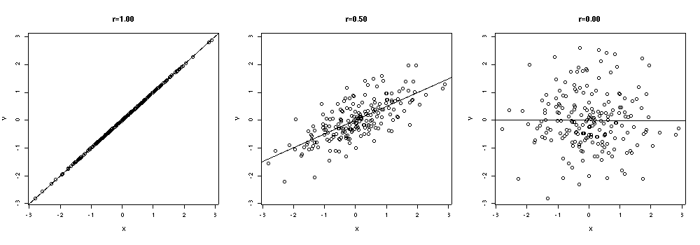
Deviations from mean divided by standard deviation (s.d.):
Correct     -1.31 -0.42 -0.12  0.48  1.37
Judge's     -1.57 -0.14  0.00  0.71  1.00
Product      2.06  0.59  0.00  0.34  1.37   sum = 3.82
Correlation = sum/4 = 0.956

Correlation of Model with Correct is almost 1

Lens model

Regression least squares demo

Dan Goldstein's demo

Judgment: Regression example

Student	P	M	F	PRE	Error
1	90	90	90	91.6	1.6
2	80	90	91	88.3	-2.7
3	70	90	84	85.0	1.0
4	70	70	71	70.7	-0.3
5	60	40	46	46.0	0.0
6	50	80	71	71.3	0.3

F = .71×M + .33×P - 2.3 + Error

Data with judgment

Student	P	M	F	J	MUD	Error
1	90	90	90	91	89.8	-1.2
2	80	90	91	84	84.9	0.9
3	70	90	84	79	80.0	1.0
4	70	70	71	70	70.0	0.0
5	60	40	46	50	50.2	0.2
6	50	80	71	66	65.2	-0.8

J = .50×M + .49×P + 0.76 + Error

Goldberg (1970, p. 423).

The clinician is not a machine. While he possesses his full share of human learning and hypothesis-generating skills, he lacks the machine's reliability. He ``has his days'': Boredom, fatigue, illness, situational and interpersonal distractions all plague him, with the result that his repeated judgments of the exact same stimulus configurations are not identical. He is subject to all those human frailties which lower the reliability of his judgments below unity. And if the judge's reliability is less than unity, there must be error in his judgments - error which can serve no other purpose but to attenuate his accuracy. If we could remove some of this human unreliability by eliminating the random error in his judgments, we should thereby increase the validity of the resulting predictions.

Regression to the mean

Nonregressiveness and representativeness

GPA prediction (Kahneman and Tversky, 1973).
Other examples: pilots, rookie of the year.

Effect reduced by thinking about missing data (Ganzach and Krantz, 1991)

But people regress on the basis of useless data:
Dilution effect (Nisbett et al., 1981)

Planning fallacy (Buehler et al., 1994)

Overattention to specific information about the case, with neglect of sources of error or variation.

Channel tunnel
expected 5 billion pounds
actual cost > 10 billion

Student thesis projects
average expected 34 days
average completion 55 days

Projects with deadlines (average 13 days)
average expected 6 days
average completion 11 days

Sydney Opera House (proposed 1957)
expected 1963 for $7 million
completed 1973 for $102 million

Sydney Opera House