Why do we overestimate others’ willingness to pay?
William J. Matthews* Ana I. Gheorghiu# Mitchell J. Callan#
People typically overestimate how much others are prepared to pay
for consumer goods and services. We investigated the extent to which
latent beliefs about others’ affluence contribute to this
overestimation. In Studies 1, 2a, and 2b we found that participants,
on average, judge the other people taking part in the study to “have
more money” and “have more disposable income” than themselves. The
extent of these beliefs positively correlated with the
overestimation of willingness to pay (WTP). Study 3 shows that the
link between income-beliefs and WTP is causal, and Studies 4, 5a,
and 5b show that it holds in a between-group design with a real
financial transaction and is unaffected by accuracy
incentives. Study 6 examines estimates of others’ income in more
detail and, in conjunction with the earlier studies, indicates that
participants’ reported beliefs about others’ affluence depend upon
the framing of the question. Together, the data indicate that
individual differences in the overestimation effect are partly due
to differing affluence-beliefs, and that an overall
affluence-estimation bias may contribute to the net tendency to
overestimate other people’s willingness to pay.
Keywords: willingness to pay, wealth-beliefs, overestimation, better-than-average effect.
1 Introduction
Price-setting, negotiation, public goods games, proxy decision-making,
and bidding in many types of auction are all situations in which
people’s behaviour is likely to be based, in part, on an estimate of
how much other people are prepared to pay for something. Recent work
indicates a widespread tendency to overestimate others’ willingness to
pay (other-WTP), and that this bias has no single cause. The present
work provides a new perspective by examining the contribution of
latent beliefs about other people’s affluence to estimates of their
willingness to pay.
1.1 Overestimating others’ willingness to pay
People systematically overestimate others’ willingness to
pay. Preliminary evidence came from van Boven, Dunning & Loewenstein
(2000), who found that sellers endowed with a product over-estimated
the amount that buyers were prepared to pay for it. More recently,
Kurt and Inman (2013) found that buyers overestimate the amount
offered by other buyers.
These findings are just one instance of a much more general result,
comprehensively established by Frederick (2012). In a first
demonstration, marketing students entered private bids for 10 products
sold via auction (Vickrey, 1961), prior to estimating the median bid
for each item. On average, estimates were 40% higher than the true
medians. This effect was robust across various procedural changes,
including: (a) giving incentives for accurate estimates, (b) asking
people to estimate the proportion of other participants who would pay
more (or less) than they would, (c) having people state their the
maximum WTP and estimate that of the next (or preceding person)
participant, or of a named acquaintance, (d) indicating whether they
would pay more or less than “the typical person taking part”, and (e)
estimating the arithmetic mean of bids in a Becker-DeGroot-Marschak
(BDM) auction (Becker, DeGroot & Marschak, 1964). However, the effect
was found to be specific to estimates of WTP, with no such
overestimation of other people’s maximum selling prices; and it is
specifically monetary, with no self-other differences in the number of
pencils that a person would be prepared to sharpen in order to earn
the product.
Notably, most of this work involved an implicit or explicit
comparison with one’s own willingness to pay (self-WTP), so that the
overestimation of WTP manifests as the belief, on average, among a
group of people that the other members would pay more than oneself: a
self-other WTP gap. This gap has also recently been found in studies
where the payment is completely at the buyer’s discretion and the good
or service is received regardless of the paid amount. Jung, Nelson,
Gneezy and Gneezy (2014) gave participants a University mug, telling
them “the mug is yours” before giving them the option to pay for
it. Participants on average estimated that the previous and next
participants would pay more than they did. In addition, some
participants were invited to “pay what you want” whereas others were
told that the mug “was paid for by the participant before you” (so
that they would be paying for the next person). The latter framing
elicited higher payments, mediated by an increase in estimates of how
much others would be paying – indicating an important role for the
(over)estimation of other-WTP in the causal chain between
price-framing and consumer decisions.
1.2 Possible explanations for the overestimation effect
Frederick (2012) tested and dismissed several explanations for the
overestimation effect. First, it does not seem to be due to people
using market price as the basis for their other-WTP judgments, because
the overestimation held for imaginary goods. Second, judgments of
whether the typical participant would like the products more or less
than oneself indicated no bias, even while participants judged that
such a person would pay more, so differences in perceived-liking are
unlikely to be responsible for the WTP gap. Third, although
participants on average reported that spending money was more painful
for them than for others, this did not predict the size of the
self-other WTP discrepancy, arguing against an “empathy gap”
explanation (van Boven et al., 2000). Fourth, although people often
report being above average on desirable traits (the “better than
average” effect; e.g., Brown, 2012), it is not clear that being less
prepared to pay for a product is desirable; moreover, making more
money from a sale presumably is desirable, but there was no self-other
gap for selling prices. A fifth possibility is that the products were
generally undesirable: if people know that they do not value the
product but are unsure about other people, they may conclude that they
value it less than average (analogous to the belief that one is below
average on a difficult task; Krueger, 1999; Moore & Cain,
2007). However, the effect never reversed in the way that this account
would predict for highly-prized products. Finally, Frederick rejected
the idea that, because other people are represented at a more abstract
level than oneself (Trope & Lieberman, 2003), “low level”
considerations such as budget and space limits are more prominent for
oneself than for others; the WTP gap was large irrespective of whether
the other was cast in abstract or concrete terms, and unaffected by
shifting the transaction outcomes into the future – which ought to
have raised the “construal level”.
The over-estimation of others’ willingness to pay is therefore likely
to be multiply-determined – so much so that Frederick (2012) labelled
it “the X effect”. One remaining possibility is that the effect partly
results from beliefs about other people’s financial
circumstances. Broadly: people may overestimate others’ willingness to
pay because they overestimate their ability to pay. The current
work explores this possibility.
1.3 The role of affluence-beliefs
Our primary interest concerns people’s beliefs about the financial
resources that others have available to spend on goods and services;
we use the label affluence to refer to this ability to pay for
products. No easily-reported economic measure fully captures this
construct. Wealth, for example, includes the value of a person’s
possessions and assets, whereas income captures monetary influx but
not existing cash reserves or fixed expenditures – and both measures
ignore access to credit. Given this complexity, our studies probe
affluence-beliefs in various ways, primarily focusing on measures of
income that are likely to be correlated with spending power,
psychologically as well as ecologically.
Our studies address three related questions. First, is the WTP
overestimation documented by Frederick (2012) robust and general?
Although Frederick’s studies were very comprehensive and consistent,
it is worth checking that the core effect generalizes to other labs,
samples, and procedures (e.g., Francis, Tanzman & Matthews, 2015;
Open Science Collaboration, 2015).
Second, do beliefs about other people’s affluence underlie beliefs
about their willingness to pay? Intuition suggests that richer people
will be prepared to pay more. We discuss the possible origins of such
a generalization, as well as the question of whether it is valid, in
the General Discussion; for now we simply note that if people hold the
lay-theory that affluence (the ability to pay) predicts willingness to
pay then different latent beliefs about the wealth of others will
partly underlie differences in the overestimation of other-WTP.
The third question is whether affluence-beliefs contribute to the
overall tendency to overestimate other-WTP (i.e., the mean
overestimation effect across participants). If there is a positive
relationship between estimated affluence and estimated WTP, net
overestimation of the former will create or enhance overestimation of
the latter (or reduce a tendency to underestimate, although
underestimation has never been observed).
The work surveyed above provides little direct evidence regarding the
role of affluence beliefs in the overestimation effect. In two
Appendices, Frederick (2012) reported the results of asking people to indicate
their relative standing “compared to others taking the survey today”
on a scale from –5 (much less than average) to +5 (much more than
average) for a wide range of measures, including “how wealthy are
you?” One study (N=104) found a mean response of –0.98 and a
correlation with the overestimation effect of –0.09; the other
(N=242) a mean response of –0.21 and a correlation of –0.11. These
correlations were not flagged as statistically significant, or discussed, but
both the means and correlations are in the direction predicted by the
idea that a latent belief that others are wealthier than oneself may
contribute to the overestimation of others’ willingness to pay.
In addition, a broad body of work gives reason for thinking that
people may often over-estimate the wealth of others. First, affluent
individuals are often highly-conspicuous (e.g., through media
depictions), and this availability is likely to lead to
overestimations of “typical” wealth – akin to the overestimated
frequency of exotic causes of death (e.g., Plous, 1993). Second,
upward social comparisons are more prevalent than downward comparisons
(e.g., Buunk, Zurriaga, Gonzalez-Roma & Subirats, 2003), perhaps as
part of a general directional construal of relative magnitudes
(Matthews & Dylman, 2014). Psychological and econometric studies
suggest that people typically compare themselves with others who are
similar to them (Wood, 1989), and that upward income comparisons are
more common/more highly weighted than downward ones (e.g., Boyce,
Brown & Moore, 2010; Clark & Senik, 2010). Upward comparisons may
imply a preoccupation with the idea that similar others are better off
than oneself, and/or increase the availability of more affluent
exemplars when estimating the wealth of a “typical other” – in turn
contributing to a net overestimation of their willingness to pay.
In summary, we investigate the robustness of the other-WTP
overestimation effect and probe whether individual differences in the
effect are partly due to differences in beliefs about others’
affluence. We also examine whether overestimation of others’ affluence
is typical, in a way that could partly account for the net
overestimation of others’ willingness to pay.
1.4 Overview of studies
We report 6 studies that examine the link between affluence-beliefs
and WTP estimates. Studies 1, 2a and 2b use a range of products and
procedures to investigate beliefs about other people’s affluence and
willingness to pay for consumer products, focusing on the self-other
WTP gap. Study 3 seeks evidence for a causal link between
affluence-beliefs and beliefs about WTP. Studies 4, 5a, and 5b use a
between-participant design in which people estimate the WTP of a
separate group of participants engaged in a “real” financial
transaction, and examines order and incentive effects. Study 6 probes
the accuracy of beliefs about other people’s affluence in more detail.
2 Study 1
Participants indicated the proportion of people taking part in the
survey who have more or less money than themselves; they then
indicated whether the amount that they would be prepared to pay for
each of 10 products was more or less than what the typical person
would pay.
2.1 Method
2.1.1 Participants
Participants took part on-line and were recruited via Amazon’s
Mechanical Turk (MTurk). Here and throughout, respondents who were
underage or did not complete the task were removed from the data set,
and only the first occurrence of each ip address was included to help
ensure data independence (ips that overlapped in time were both
excluded; e.g., Matthews, 2012; all exclusions were prior to
analysis). The final dataset comprised 190 participants (71 female)
aged 18–67 (M = 31.7, SD = 9.1).
2.1.2 Design and procedure
After initial instructions, participants were randomly assigned either
to “estimate the proportion of people taking part in the survey who
have more money than you do” (n = 97) or the proportion who “have less
money than you do” (n = 93), and typed their estimate in a text
box. Responses to the “less than” version were subtracted from 100 to
give the implied percentage of other people believed to have more
money than the participant.
The next webpage presented a list of 10 products (Table 1). For each,
the participant indicated whether the amount they would be willing to
pay is more or less than what “the typical person taking this survey
today would be willing to pay” (product order and left-right
assignment of the “less” and “more” response options were randomized).
Table 1: Proportion of participants who indicated that the “typical participant” would pay more than they would for each product in Study 1.
Product
P(other > self)
A freshly-squeezed glass of apple juice
.695
A Parker ballpoint pen
.863
A pair of Bose noise-cancelling headphones
.705
A voucher giving dinner for two at Applebee’s
.853
A 16 Oz jar of Planters dry-roasted peanuts
.774
A one-month movie pass
.800
An Ikea desk lamp
.863
A Casio digital watch
.900
A large, ripe pineapple
.674
A handmade wooden chess set
.732
Note: All binomial test p-values <.001.
A subsequent page asked for demographic information: age, gender, and
annual pre-tax household income with 8 categorical options: Less than
$15,000; $15,001–$25,000; $25,001–$35,000; $35,001–$50,000;
$50,001–$75,000; $75,001–$100,000; $100,001–$150,000; greater
than $150,000 (e.g., Kraus, Adler & Chen, 2013). Income responses
were converted into estimates of absolute income using a median-based
Pareto-curve estimator (Parker & Fenwick, 1983).1.
These demographic control variables were included in all studies.
2.2 Results and discussion
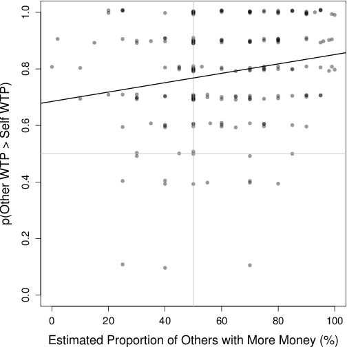
Figure 1 provides a simple illustration of the data by plotting the
proportion of products for which the participant judged that other
people would pay more against the participant’s estimate of the
proportion of participants who have more money than them. The figure
illustrates three core findings.
Figure 1: Results of Study 1. The plot shows the proportion of
products for which the participant judged that the typical
participant would pay more than they would against the
participant’s estimate of the percentage of others who have more
money than they do. y-axis values have been jittered to reduce
overplotting.
First, participants judged that others would pay more for a majority
of products (the data cluster in the top half of the plot). Table 1
confirms that, for every product, the majority of participants
believed that others would pay more than they would.
Second, participants typically judged their own wealth to be below
that of most other participants (the data cluster in the right-hand
side of the plot). Specifically, 57.3% of participants believed that
they had less money than the median; only 22.6% judged that they had
more. Participants on average believed that 61.0% (SD = 22.4%) of
other people had more money than they did, (95% CI = 57.8%, 64.2%)
t(189) = 6.73, p<.001. This result was unaffected by the wording
of the relative wealth question (Mlessthan = 62.9%,
SD = 22.8%; Mmorethan = 59.1%, SD = 22.0%;
t(188) = 1.15, p = .250).
Third, the WTP gap was positively related to affluence judgments, as
evinced by the upward-sloping regression line. To test this
relationship formally, we used mixed effects logistic regression using
the lme4 package (Bates, Mächler, Bolker, & Walker, 2015) for the R statistical language.
The dependent variable was whether the participant believed that the
typical person would be willing to pay more for the product (coded 1)
or not (coded 0); the key predictor variable was PMORE, the
participants’ estimates of the proportion of other people with more
money than them; we subtracted 50 from each value so that 0 implies
the belief that an equal number of people are more/less affluent than
oneself, and used this variable (labelled c.PMORE) in the analysis. We
also included PHRASING (whether the participant estimated the
proportion with less money or more money) and its interaction with
c.PMORE. Age, Gender (0=Male 1=Female), and household income were
included as control variables (after standardization by
z-scoring). We included random intercepts for participants and
products, and random slopes by product for the effect of c.PMORE
(Barr, Levy, Scheepers & Tily, 2013). The fixed effects are reported
in Table 2; participants with lower perceived relative wealth were
more likely to judge other people as willing to pay more for the
products; no other predictors are significant, apart from the
intercept. The positive intercept means that participants who judged
their own wealth to be at the median of the sample (and who were
average on the control variables) believed that others would typically
pay more than them.
Table 2: Fixed effects coefficients and 95% confidence intervals from
mixed effects logistic regression for Study 1.
Predictor
Coef.
CIlower
CIupper
z
p
Intercept
1.483
1.126
1.841
8.13
<.001
c.PMORE
0.012
0.002
0.022
2.27
0.024
z.PHRASING
0.077
-0.122
0.275
0.76
0.450
z.PHRASING * c.PMORE
0.004
-0.004
0.012
0.97
0.331
z.INCOME
-0.126
-0.324
0.072
1.25
0.213
z.AGE
-0.039
-0.227
0.149
0.41
0.685
z.GENDER
0.149
-0.040
0.338
1.54
0.123
How important is this effect? Using the regression parameter
estimates, the odds of judging that the next person will pay more than
oneself increase by approximately 14% when PMORE increases from 50%
(the belief that one’s own wealth is right in the middle of the sample
distribution) to 61% (the mean response for this sample). Calculating
effect sizes is non-trivial for mixed-effects logistic regression, but
the simple correlation depicted in Figure 1 has r=.200: beliefs
about the proportion of more affluent others accounts for about 4% of
the variance in the WTP effect — a "small to medium" effect, as one
might expect for such a multiply-determined and noisy outcome as
stated/estimated WTP.2 As noted in the Introduction, previous work
in this area has largely established factors that do not
contribute to the overestimation effect (Frederick, 2012), so finding a factor that makes even a modest contribution has some value.
In summary, participants tended to believe that the majority of other
participants have more money than they do and that other participants
would pay more for each product than they would. The strength of these
two beliefs was positively related: affluence-beliefs accounted for
individual differences in the WTP overestimation effect, and are
likely to contribute to the net effect. However, the belief that
others would pay more was not entirely due to the belief
that they are more affluent.
3 Studies 2a and 2b
Studies 2a and 2b built on Study 1 by changing the way that
people indicated their subjective relative discretionary income
(SRDI), and having them actually state their WTP for various consumer
products in dollars and cents before stating the WTP of other
people. Studies 2a and 2b differed from one another only in the order
of the tasks.
3.1 Method
3.1.1 Participants
For Study 2a participants were recruited via MTurk; those whose IDs/ip
addresses occurred in Study 1 were excluded giving N = 408 (240
female, ages 18-75, M = 37.4, SD = 12.1) For Study 2b participants were
recruited via the Crowdflower participant-recruitment platform
(www.crowdflower.com/pricing) giving N = 381 (230 female, ages
18-70, M = 36.9, SD = 12.1).
3.1.2 Design and procedure
In Study 2a, participants first indicated how their discretionary
income [“the amount you have to spend as you wish after paying taxes
and unavoidable outgoings (e.g., bills/mortgage/rent)”] compares with
that of “the next person who will take this survey”. As in Frederick
(2012) this framing is a way of getting people to think of a specific
individual who is representative of the other participants in the
study. Participants made their judgments on a 9-point scale: “Mine is
very much lower”; “Mine is much lower”; “Mine is somewhat lower”;
“Mine is slightly lower”; “They are exactly the same”; “Mine is
slightly higher”; …”Mine is very much higher”. We coded these from +4 to
–4, respectively, such that zero corresponded to equal affluence, and
increasingly positive numbers correspond to a belief that the other
person is progressively more affluent than oneself.
On the next page participants were asked to imagine that they are
attending an auction for consumer products and that they would have to
state the most that they would be willing to pay for the product prior
to price revelation. (Full instructions for this and other studies
using auction-type tasks are included in the
Supplement.)
Examples were used to show how under-stating or over-stating one’s
maximum willingness to pay would lead to sub-optimal outcomes, such that “you
should be absolutely honest about how much you would be willing to pay
— do not under- or over-state the amount”.
The next 10 pages presented, in random order, 10 consumer products (listed in Table 3) with photographs, and asked (for example),
“What is the maximum that you would be willing to pay for this 3 lb
jar of jelly beans?” Participants typed a numeric value in dollars and
cents before progressing to the next product. After responding to all 10 products, the task was repeated
but participants had to indicate the maximum that
“the next person to take this survey would be willing to pay” for each item. Finally, participants reported demographic information.
Table 3: Geometric means for Self- and Other-WTP values in Studies 2a and 2b.
Study 2a
Study 2b
Self
Other
t (df)
Self
Other
t (df)
A 3 lb jar of jelly beans
6.61
9.83
11.95 (405)
7.67
10.28
9.89 (375)
A 7" Kindle Fire
93.97
122.60
9.47 (405)
104.67
121.99
8.06 (358)
A 14" gemstone globe
42.81
71.50
8.82 (404)
45.50
61.21
6.14 (375)
A Bissell bagless vacuum cleaner
83.78
114.20
10.71 (405)
84.01
113.77
8.97 (368)
A box of 40 deluxe Belgian chocolate
15.87
22.07
10.78 (403)
15.69
20.28
9.50 (377)
A leather-bound notebook
14.04
21.87
10.43 (397)
12.69
16.81
9.02 (369)
A National Geographic Atlas of the World
14.42
20.90
9.58 (404)
12.63
16.34
7.48 (366)
A Samsung Galaxy Gear Smartwatch
77.42
126.85
12.39 (403)
78.88
118.70
11.14 (378)
A one-year subscription to Scientific American
12.20
17.79
9.68 (403)
10.83
15.86
8.30 (372)
A TomTom SatNav with Lifetime Maps
59.98
101.54
12.18 (397)
67.33
97.89
8.33 (371)
Note: t’s are for paired-samples tests comparing log-transformed Self and Other WTP values. All p’s <.001.
Study 2b was identical except that participants answered the question
about subjective relative discretionary income after the WTP
judgments.
3.2 Results and discussion
These and subsequent studies involved free estimates of own/others’
WTP. Such data are typically positively skewed and include a handful
of extreme values (e.g., Walasek, Matthews & Rakow, in press). We
screened for outliers using the boxplot-based procedure for skewed
distributions proposed by Hubert and Vandervieren (2004) and
implemented by the adjbox function for the R statistical language
(Rousseeuw et al., 2015), and removed responses that were more than
three times the interquartile range away from the edges of the
box. This led to removal of 48 observations (0.6%) in Study 2a and
109 observations (1.4%) in Study 2b. WTP estimates were
log-transformed to help symmetrize the data. (Here and throughout,
log-transformation was ln(x+1), to deal with possible zero values.)
We calculated the WTP gap (other-WTP minus self-WTP after
log-transformation of each); more positive values indicate a stronger
tendency to believe that others would pay more than oneself.
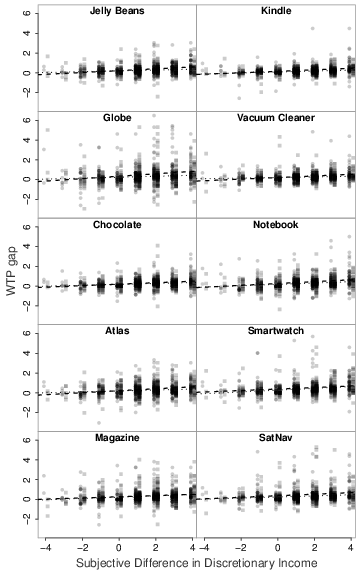
Figure 2 plots the WTP gap against subjective difference in
discretionary income for each of the 10 products; larger values on the
y-axis imply greater overestimation of others’ WTP; larger values on
the x-axis imply stronger belief that the other person is more
affluent than oneself. The data from Study 2a are shown by circles;
those from Study 2b are plotted as squares (the x-axis values have
been offset slightly to separate the two data sets).
Figure 2: The relationship between WTP gap and subjective affluence
difference for each product in Studies 2a and 2b. x-axis values have been offset slightly to separate the
two data sets (Study 2a = circles; Study 2b = squares). The lines
show simple regression lines for Study 2a (dashed) and Study 2b
(dotted).
The plots illustrate the same effects as Study 1. First, the majority
of participants believed that the next person’s discretionary income
is higher than their own (the data cluster in the right-hand side of
each panel). In Study 2a the response to the discretionary income
question (M= 1.42, SD = 1.85) was well above the value of 0
expected if people judged the next person’s income to match their own,
t(407) = 15.51, p<.001 The results from Study 2b were very
similar, M = 1.26, SD = 1.69, t(380) = 14.51, p <.001.
Second, most participants believed that other people would pay more
for each product than they would (the data cluster above y=0). Table
3 confirms that, for all products, participants on average estimated
the next person’s WTP as substantially above their own.
Finally, the greater the subjective difference in affluence, the
greater the WTP gap: participants who judged the next person to have
much higher discretionary income than themselves also believed that
the other person would pay considerably more for each product,
illustrated by the simple regression lines (the dashed and dotted
diagonal lines are for Studies 2a and 2b, respectively). The top
section of Table 4 shows the results of fitting a mixed-effects model
akin to that from Study 1, with fixed effects for subjective
difference in discretionary income (SDDI) and the demographic
variables household income, age, and gender; random effects for
participant, product, and by-product random slopes for the effects of
SDDI. (Here and in subsequent studies using linear mixed effects
modelling, p-values are based on Satterthwaite’s approximation and
were computed using the lmerTest package for R; Kuznetsova, Brockhoff
& Christensen, 2014.)
In both studies the WTP-gap is positively related to SDDI, confirming
the impression from Figure 2. We calculated marginal R2 values
using the approach for the fixed effects component of mixed effects
models described by Johnson (2014) and Nakagawa and Schielzeth (2013)
using the MuMIn package for R (Barton, 2015; for simplicity the
control variables were excluded). The values were .044 and .019 for
Studies 2a and 2b, respectively. The effect is present irrespective of
whether people indicated their relative affluence before or after
making the WTP judgment; it seems to be slightly weaker in the latter case
(Study 2b), but the change in participant populations between studies
makes direct comparison impossible. Study 2b also shows an independent
and rather counter-intuitive effect of household income on the WTP
gap, with higher incomes predicting a greater belief that the next
person would pay more than oneself.
Table 4: Fixed effects for Studies 2a and 2b.
Study 2a
Study 2b
Predictor
Coef.
CIlower
CIupper
t (df)
p
Coef.
CIlower
CIupper
t (df)
p
WTP-gap
Intercept
0.241
0.163
0.320
6.03 (43.7)
<.001
0.200
0.141
0.258
6.71 (52.1)
<.001
SDDI
0.095
0.065
0.124
6.32 (220.7)
<.001
0.064
0.037
0.090
4.74 (99.1)
<.001
z.INCOME
0.029
-0.024
0.081
1.06 (397.7)
0.291
0.053
0.011
0.095
2.48 (373.4)
0.014
z.AGE
-0.033
-0.080
0.014
-1.36 (398.7)
0.174
0.006
-0.034
0.045
0.28 (374.2)
0.780
z.GENDER
-0.008
-0.056
0.039
-0.35 (398.6)
0.729
0.017
-0.022
0.057
0.86 (373.6)
0.392
Self
Intercept
3.480
2.899
4.061
11.74 (9.3)
<.001
3.476
2.869
4.084
11.22 (9.2)
<.001
SDDI
-0.045
-0.081
-0.010
2.52 (247.1)
0.013
-0.044
-0.083
-0.004
2.17 (122.5)
0.032
z.INCOME
-0.017
-0.081
0.047
0.52 (401.6)
0.605
-0.029
-0.090
0.034
0.88 (374.2)
0.378
z.AGE
0.002
-0.055
0.059
0.08 (402.2)
0.939
0.018
-0.040
0.077
0.61 (374.7)
0.542
z.GENDER
0.0267
-0.031
0.084
0.91 (401.8)
0.362
0.027
-0.032
0.086
0.88 (374.2)
0.377
Other
Intercept
3.727
3.134
4.32
12.32 (9.1)
<.001
3.682
3.074
4.290
11.87 (9.1)
<.001
SDDI
0.049
0.020
0.077
3.37 (90.3)
0.001
0.018
-0.011
0.048
1.21 (169.1)
0.227
z.INCOME
0.009
-0.038
0.056
0.37 (396.2)
0.709
0.020
-0.029
0.069
0.79 (366.8)
0.429
z.AGE
-0.029
-0.071
0.013
1.37 (396.4)
0.171
0.022
-0.025
0.068
0.92 (366.3)
0.358
z.GENDER
0.018
-0.024
0.060
0.86 (396.8)
0.392
0.041
-0.005
0.088
1.73 (366.6)
0.084
Note: SDDI = Subjective Relative Discretionary Income. df and p-values based on Satterthwaite approximation.
Notably, the intercepts are significantly above zero, implying that
even participants who judge their own discretionary income to be
identical to the next person’s believe that the next person would be
willing to pay more.
We repeated these regression analyses but with Self-WTP and Other-WTP
as separate outcome variables (see Table 4; marginal R2 calculated
as above were .003 and .005 for the Self and Other data of Study 2a,
and .002 and .001 for Study 2b). In both studies, participants who
believed themselves relatively better off had higher WTP for the
products. In Study 2a, participants who regarded themselves as less
affluent also gave higher estimates of the next person’s WTP; the
effect in Study 2b was in the same direction but not significant. No
other predictors were significant — including household
income. Thus, participants’ willingness to pay was better predicted by
their sense of their relative affluence than by a (rather crude)
objective measure of spending power.
Using these regression models, we calculated the expected Self-WTP and
Other-WTP (across all products) for participants who believed their
own wealth to exactly equal the next person’s: the values were
$32.46 (self) and $41.55 (other) in Study 2a, and $32.33 (self) and
$39.73 (other) in Study 2b, giving WTP gaps of $9.09 and $7.40,
respectively. Computing the same expectations for participants at the
mean value of the comparative-affluence question (recall that
participants on average believed that they were worse off than their
peers) yielded self-other gaps of $14.10 (and increase of 55%) and
$10.05 (and increase of 36%) for Studies 2a and 2b, respectively.
We conducted two additional analyses. First, we repeated the analysis
of the Self-WTP data but this time without including subjective
relative discretionary income as a predictor, in order to further examine whether
actual household income predicted people’s product valuations. There
was no indication of an effect for either study (for Study 2a, the
coefficient was 0.022, 95% CI: –0.035, 0.079; for Study 2b it was
–0.004, 95% CI: –0.063, 0.055; the results were virtually identical
when we allowed the slopes to vary randomly across products). Thus, we
found little indication that people’s actual affluence (albeit rather
crudely measured) predicted their willingness to pay for the products
studied here.
Second, we plotted the other-WTP estimates against self-WTP
values. For every product in both studies, participants with higher
self-WTP reported higher other-WTP (all Pearson’s r > .47, all
p <.001), consistent with the possibility that people partly base
their judgments of others’ WTP on their own WTP. In addition, the
regression lines were swivelled towards the horizontal (coefficients
ranged from 0.310 to 0.651; M=0.498) in keeping with the central
tendency of judgment seen in many domains, including price judgments
(e.g., Matthews & Stewart, 2009). This might be a simple consequence
of error in the predictor variable (the “error in variables”
problem). An alternative (not mutually exclusive) possibility is that
people partly base their other-WTP estimates on their own WTP, but
that they take into account the extremity of their valuations and
guess something closer to the mean of the distribution.
4 Study 3
Study 3 sought to establish a causal link between beliefs about
others’ affluence and beliefs about their willingness to pay.
4.1 Method
4.1.1 Participants
Participants were recruited via MTurk. IDs/ip addresses that had taken
part in Studies 1 or 2a were excluded leaving a sample of 311 (117
female, ages 18–69, M = 34.5, SD = 10.8).
4.1.2 Design and procedure
Participants were asked to think about a person who is attending a
special kind of auction for various consumer products, with
instructions similar to Studies 2a and 2b. On the next page,
participants were randomly assigned to a “low income” condition
(N = 155) or a “high income” condition (N = 156), such that they
were told that the person taking part in the auction has a personal
income of $10,000 [$60,000] per year, “which puts them in about the
bottom [top] 20% of people in the US”.
The following 10 pages each showed a product image and description,
and asked: “What would the person bid (i.e., what is the most that
they would be prepared to pay) for this…”. Table 5 lists the
products. Participants entered their responses in a text box. Product
order was randomized, but a software error meant that the “blender”
came first for most participants. Finally, participants entered
demographic information.
4.2 Results and discussion
Forty responses (1.3%) were excluded as outliers (their inclusion did
not affect the pattern of significance). Table 5 shows the geometric
means and results of independent-sample t-tests for every
product. In all cases, estimated WTP was higher in the high-income
condition than in the low-income condition.
Explicitly stating the other person’s income in this way might entail
demand characteristics, a concern which could partly — but probably
never fully — be ameliorated by rendering the other’s affluence more
subtly (for example, by presenting a character sketch and having
people estimate the individual’s salary on a scale whose set of values
imply a high or low income). Nonetheless, the data provide reasonable
evidence that beliefs about another person’s affluence causally affect
beliefs about their willingness to pay for consumer products.
Table 5: Geometric means for the Low- and High-income conditions of Study 3.
Product
Low
High
t (df)
10 oz French Vanilla Scented Candle
4.70
9.97
11.05 (307)
30" x 60" Beach Towel
5.84
10.20
8.62 (286)
DecoMates Wall Clock
9.65
20.48
10.16 (309)
Fiskars Big Grip Trowel
5.39
10.91
10.17 (279)
George Foreman Family-Size Grill
29.05
48.78
7.81 (306)
Hamilton Beach Multi-function Blender
26.12
56.24
11.56 (308)
Heavenly Honeycomb 12" Chocolate Pizza
8.70
14.87
9.26 (298)
Hooded Sweatshirt
13.74
21.53
7.96 (286)
Nokia Lumia 920 32Gb 4G Phone
105.66
191.94
7.46 (309)
Canon 16.1 Megapixel Digital SLR Camera
127.20
281.66
8.84 (286)
Note: All p< .001. df were Welch-corrected where necessary and are rounded to nearest integer.
5 Study 4
We next investigated whether the relationship between affluence
beliefs and WTP estimates applied in a between-group design, where one
set of participants estimated the valuations of another group. We also
sought to generalize the preceding results by having participants
estimate other people’s pre-tax incomes on a dollar scale, and with
people making judgments about a real financial transaction under
accuracy incentives.
Study 4 served as pilot for Studies 5a and 5b. Participants were told
about a study of consumer behaviour in which 20 adults had been
recruited to take part in a Vickrey second-price auction. The
participants estimated both the average annual income of this
(hypothetical) sample of 20 people, and the average of the 20 bids
that would be submitted in the auction.
5.1 Methods
5.1.1 Participants
The final sample comprised 389 (145
female, ages 18–70, M = 34.2, SD = 11.8) recruited via MTurk. The
lapse of time and change of task meant that we did not screen for
participation in earlier studies.
5.1.2 Design and procedure
Participants were asked to suppose that the experimenter is going to
recruit a sample of 20 participants for a study looking at spending
behaviour, and that these participants will “be a mixture of staff and
students at the University where I work. The people will be a mix of
men and women, and none of them will be under 18 or over 60 years of
age. All of them will have a regular income.”
Participants then completed two tasks. In one, they estimated the
average of the annual pre-tax income of the 20 people in the sample,
to the nearest thousand dollars per year, by moving a slider whose
range spanned 0 to 200 (with responses multiplied by 1000 for
analysis). In the other task, they were informed that the 20 people
would take part in an auction for a “Hotel Chocolat” Dinner Party
Hamper. This product was pictured and fully described, and on the next
page participants read the instructions for the auction: each person
would submit a private bid; the highest bidder would win, and
would pay the value of the second-highest bid. It was explained that
the optimal strategy is to bid exactly the maximum that one is willing
to pay for the item. Participants then estimated the average amount
that would be bid for the hamper. The order of the income-estimation
and bid-estimation tasks was randomized.
Participants next used a slider to indicate the number of people that
were to be recruited for the auction as an attention/memory
check. Finally, they entered demographic information.
5.2 Results and discussion
Twenty three participants (5.9%) failed the attention check and were
excluded. Six participants (1.6%) were excluded because of outlying
WTP and/or income estimates. Log-transformed WTP estimates served as
the dependent variable in a linear regression with estimated income
(ESTINC) as the key predictor. The regression model also included
task order (ORDER, coded 0 when WTP estimate preceded income estimate
and 1 when the order was the opposite) and its interaction with income
estimate; gender; age; and own household income. All predictors were
standardized (the interaction term was computed from the standardized variables and was not itself standardized) and all variables were entered simultaneously.
The results are shown in Table 6. The key finding is that WTP
estimates were positively related to income estimates
(Δ R2 = .050; Curtin, 2015); in addition, WTP estimates
increased with participant age. Repeating the analysis with outlying
responses included had little effect on the coefficients except that
age was no longer significant. Repeating the analysis including the
participants who failed the attention check had very little effect on
the coefficients, except for a weak tendency for women to produce
larger estimates than men (b = 0.082, p = .032).
Table 6: Regression analyses for Studies 4–5b.
Predictor
Coef.
CIlower
CIupper
t
p
4
Intercept
3.889
3.814
3.964
102
<.001
z.ESTINC
0.174
0.097
0.252
4.41
<.001
z.ORDER
0.022
-0.053
0.098
0.58
0.564
z.ORDER* z.ESTINC
0.005
-0.071
0.080
0.12
0.902
z.AGE
0.114
0.038
0.190
2.96
0.003
z.GENDER
0.067
-0.009
0.143
1.75
0.082
z.INCOME
-0.038
-0.116
0.039
0.98
0.33
5a
Intercept
3.009
2.95
3.068
101
<.001
z.ESTINC
0.062
0.001
0.122
1.99
0.047
z.SAMPLE
0.035
-0.027
0.097
1.12
0.265
z.ORDER* z.ESTINC
-0.029
-0.085
0.027
1.02
0.308
z.AGE
0.041
-0.019
0.101
1.33
0.183
z.GENDER
-0.042
-0.102
0.017
1.40
0.164
z.INCOME
-0.019
-0.079
0.041
0.62
0.538
5b
Intercept
2.934
2.879
2.989
106
<.001
z.ESTINC
0.085
0.027
0.142
2.88
0.004
z.INCENT
0.047
-0.007
0.102
1.70
0.089
z.INCENT* z.ESTINC
-0.004
-0.059
0.050
0.16
0.872
z.AGE
-0.049
-0.104
0.007
1.73
0.084
z.GENDER
0.021
-0.034
0.076
0.74
0.458
z.INCOME
-0.041
-0.099
0.017
1.38
0.169
Note: See text for definition of predictors. t-values greater than 100 rounded to nearest integer.
6 Studies 5a and 5b
Studies 5a and 5b replicated Experiment 4 but using a real financial
transaction and accuracy incentives.
6.1 Auction
First, 25 employees of the University of Essex (14 female, ages 22–54,
M= 36.0, SD = 10.0) were paid £5 to take part in an auction. They
completed a computer-based task in individual cubicles. They learned
that they were taking part in an auction for a “Chocolate Lovers Gift
Hamper”, and were shown a picture and full description of this product
(retail price excluding delivery £38.25). The instructions for the
Vickrey auction were similar to those of Study 4, and explained that
participants should indicate the most that they would be prepared to
pay for the product. It was emphasized that the auction was real that
participants could submit bids that were as little or as much as they
liked (including zero).
After submitting their bid they provided demographic information,
including their annual pre-tax income (reported as an exact numerical
amount; anonymity of data storage was assured). Participants were
asked not to discuss their bid with anyone else.
6.2 Results
The winning bid was £28.50, and the winner paid the second-highest
value of £21.00. The mean, median and SD of the bids and
self-reported incomes are shown in Table 7. Both variables were
positively skewed, particularly the bid values. Income and WTP were
uncorrelated, r = 0.13 [95% CI: −0.279, 0.500], t(23) = 0.63,
p = .534 [Spearman’s ρ = .171, p = .413].
Table 7: Actual and estimated bids and incomes for the auction used in Studies 5a and 5b.
Incomes
Bids
M
SD
Mdn
M
SD
Mdn
Auction
£24,398
£12,586
£21,500
£9.56
£7.95
£7.00
Study 5a
£26,248
£9,298
£25,000
£23.43
£15.91
£20.00
Study 5b
£28,077
£9,397
£27,246
£23.30
£18.84
£19.56
Note: "Auction" refers to the real responses of the sample recruited to take part in the auction. Responses from Study 5b have been converted to pounds Sterling.
6.3 Main experiments
Study 5a was very similar to Study 4, except that (a) the participants
were (like the participants in the auction) based in the United
Kingdom, (b) they were asked to estimate the incomes and WTP for the
real auction rather than a hypothetical one, (c) they were given an
incentive for accuracy, and (d) they estimated incomes by entering a
free-text response rather than adjusting a slider.
The data from Study 5a were somewhat noisy; Study 5b was a replication
which used a U.S. sample and which manipulated accuracy incentive.
6.4 Methods
6.4.1 Participants
In Study 5a, a total sample of 556
participants (363 female, ages 16–64, M = 26.8, SD = 9.3) was
obtained from two sources in parallel: 385 were recruited from the
“Prolific Academic” on-line recruitment tool, pre-selected to be
resident in the U.K.; the remaining 171 were staff and students at the
University of Essex, recruited via an email to the University
participant panel. For Study 5b participants were recruited via MTurk
(those whose ids/ips had been used for Study 4 were excluded); the
sample comprised 837 participants (328 female, ages 18–77, M = 32.9,
SD = 10.7).
6.4.2 Design and procedure
In Study 5a participants were told that we had recruited a sample of
25 employees from a British University to take part in an auction for
the chocolate hamper. The instructions and task were similar to Study
4, except that (a) the auction was no longer presented as
hypothetical/in the future, and (b) participants were told that there
would be a £10 bonus for the most accurate response to each of the two
questions that they would be asked.
Participants first estimated “the average (arithmetic mean)” annual
pre-tax income of the 25 auction participants (entering their response
as a free numeric value). They were then given a copy of the
instructions that the auction-participants had seen and estimated the
average of the 25 bids. They subsequently completed the
attention/memory check from Study 4 – which we label the “sample size
check” — as well as an additional 4-alternative multiple choice
question about the rule for deciding who would win the auction and how
much they would pay – which we label the “auction rules
check”. Finally, they provided demographic information; the response
categories for the question about about own annual household income
were converted into pounds Sterling.)
Study 5b was identical except that: (a) the sample of 25
auction-participants were described as being recruited from “a
University” (rather than a British University), (b) approximately half
(N = 406) were given the accuracy incentive: they were told that
there would be a $15 dollar reward for the most accurate response to
each of the two estimates; the remaining participants received
identical instructions but without this information. Participants’
responses were converted into Sterling using the exchange rate from
the day of the study, and the debriefing explained that the original
auction was run in the U.K., and that the participants’ responses would
be converted into Sterling when determining their accuracy.
6.5 Results and Discussion
6.5.1 Study 5a
Seventy five participants (13.5%) incorrectly answered the
sample-size check question and were excluded. A further 26 (5.4%)
were excluded because of outlying WTP and/or income estimates, leaving
a final sample of 455.
Descriptive statistics are shown in Table 7, which shows that mean
estimated average WTP (i.e., the average bid) was more than twice the
true value. To compare the estimated average WTP with the average
produced by the participants in the auction, one may either treat the
latter as a single, fixed value using a one-sample t-test or
acknowledge that, even though our auction produced a single “true”
mean, this will be subject to sampling error so that it is more
appropriate to use a Welch t-test to compare the mean of the average
WTP estimates with the mean of the true WTP values. We took the latter
approach (using ln(x+1) for both data sets) and found a significant
difference between estimated and actual average WTP, t(25) = 4.97,
p < .001.
The mean estimated average income was approximately 7.5% greater than
the true value, a difference that was not significant,
t(25.46) = 0.72, p = .476. (As noted above, the true
auction-goers’ data were positively skewed; there was much less skew in
the estimates, so neither set was transformed for this analysis.) The
median values show the same modest overestimation of income as the
means.
The WTP estimates were submitted to a regression analysis with
participants’ estimates of the auction-goers’ incomes (ESTINC) as the
key predictor of interest. Participant sample (SAMPLE: Prolific
Academic vs. University of Essex, coded 0 and 1 respectively) and its
interaction with income estimate as well as the demographic variables
gender, age, and participants’ own household income were included as
predictors (with standardization as for Study 4). The results
are shown in Table 6.
Participants’ estimates of mean auction bids were positively related
to their estimates of mean income. However, although the effect is
significant, it is weak (Δ R2 = .009) – and noticeably weaker
than in Study 4. Repeating the analysis with extreme values included
rendered the effect of income-estimates non-significant (b=0.053,
p = .479) and led to age being a weak but significant positive
predictor (b=0.088, p=.022). Noticeably, the outlying responses
include values which exert great influence and are almost certainly
typos – e.g., estimated average bids of £2500 and estimated average
income of £1 per year.
We also re-ran the analysis without excluding participants who failed
the sample-size check (but with outlier screening); the pattern
mirrored the main analysis, with a slightly larger effect of estimated
mean-income (b = 0.075, p = 0.011). Finally, we re-ran the
analysis using only those participants who passed both the sample-size
check and the auction-rule check (again, with outlier screening; final
sample size = 371). The results were similar to the main analysis,
except that the effect of income estimates, while still positive, was
no longer significant (b = 0.050, p = .147).
Taken together, the data suggest a weak positive relationship between
people’s estimates of the auction-goers’ mean income and the estimates
of the mean bid in the auction. However, the finding is not
convincing, particularly when compared with Study 4.
6.5.2 Study 5b
A total of 84 participants (10.0%) incorrectly answered the
sample-size check question and were excluded (43 from the incentive
condition, 41 from the no-incentive condition). A further 21 (2.8%)
produced outlying income and/or WTP estimates and were also excluded,
leaving a final sample of 732 (382 in the no-incentive condition, 350
in the incentive condition).
As shown in Table 7, the mean estimated average WTP (after converting
WTP and income estimates to Sterling) was again more than twice the
value of the true mean, t(24.87) = 4.60, p < .001. The mean
estimated average income was approximately 15% greater than the true
value, although the difference was not significant, t(24.92) = 1.45,
p = .160. The American participants in this study probably based
their WTP and income estimates on U.S. norms, which are likely to
differ from those in the U.K., where the auction was conducted.
As in Study 5a, we regressed log-transformed estimates of average WTP
onto estimated annual incomes; we included incentive condition
(INCENT, coded 0 for no incentive and 1 for incentive) and its
interaction with income estimate, as well as age, gender, and own
household income, as predictors (Table 6). Estimated average bids were
positively related to estimated average incomes (Δ R2 =
.112). Repeating the analysis with outliers included led to very
similar results, except that WTP estimates were now significantly
larger when participants were given an incentive for accuracy
(b = 0.062, p = .037). Re-running the original analysis without
excluding participants who failed the sample-size check had no effect
on the pattern of significance and slightly increased the size of the
effect of income estimate (b=0.101, p <.001). Finally, we re-ran
the analysis using only those participants who passed both the
sample-size check and the auction-rule check; the results mirrored the
main analysis except that the negative relationship between
participant age and WTP estimates was now significant (b=−0.065,
p = .027).
In short, this study confirmed the rather weak effect found in Study
5a and establishes that affluence-beliefs predict estimates of others’
WTP in a between-group design: estimated average WTP was positively
related to estimated average income. There was no indication that
accuracy incentives modulated this effect or altered engagement with
the task.
7 Experiment 6
This experiment sought a clearer understanding of how people judge
their own wealth relative to others. In a very simple task,
participants reported their own annual income and estimated that of
the next person to take part in the study.
7.1 Method
7.1.1 Participants
A sample of 433 participants (273 male,
ages 18-72, M = 31.8, SD = 9.9) were recruited via MTurk. (This
study was conducted after Study 3 but before Studies 4-5; because the
task is quite different from the WTP judgments of earlier studies,
participants were not screened for participation in these studies.)
7.1.2 Design and Procedure
On one page participants were
asked to “think about the next person who will complete this
survey. What is your best estimate of their annual pre-tax income?
(That is, how much do they make each year, before taxes?”) and typed
their judgment in a text box. A separate page used identical wording
but asked about “your own” pre-tax income. The order of the tasks was
randomized (217 participants reported “self income” first; 216
estimated “other income” first). Participants then reported their
gender and age.
7.2 Results and discussion
Seven participants (1.6%) were excluded for producing outlying
responses (1 for “self-income”; 6 for “other-income”).
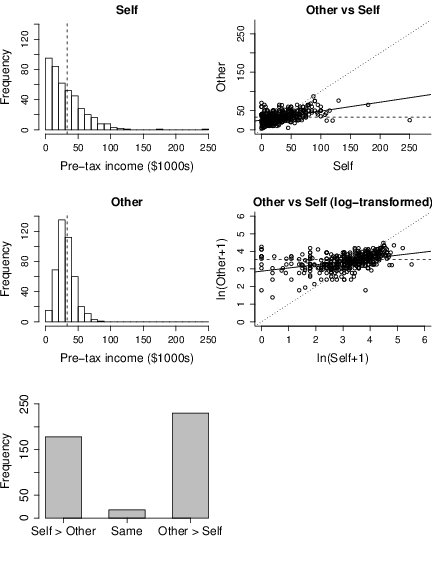
The top left panel of Figure 3 shows the distribution of participants’
incomes; the vertical dashed line shows the arithmetic mean of
$33,101 (SD = 28,483). The next panel down shows the distribution
of estimated incomes; this is less positively skewed, with an
arithmetic mean of $33,121 (SD = 13,709). A paired t-test found
that participants’ estimates of the next person’s income did not, on
average, differ from their self-reported income, t(425) = 0.02,
p = .987. In other words, the average estimate of the next person’s
income almost exactly matches the true expected value of that income.
Figure 3: Results for Study 6. Left hand panels: distribution of
self-reported annual pre-tax incomes (Self) and estimates of the
next person’s income (Other); vertical dashed lines show the
distribution means, which are very similar; the bottom panel shows the number of
participants judging the next person as having lower, higher, or
the same income as them. Right-hand panels show the relationship
between judgments of the next person’s income and the
participant’s own income. The solid lines are OLS regression
lines; the dashed lines show performance if participants perfectly
reported the expected value of the next person’s income (i.e., the
mean of the self-reported income values); the dotted line shows
performance if participants indicated that others’ income exactly
matched their own.
However, because the true income distribution is positively skewed,
the majority of participants (58.2%) have incomes which are below the
mean. The bottom left panel of Figure 3 shows the number of
participants who judged their own income to be greater than, the same
as, or less than that of the next person; the proportion who indicated
that the next person would have a higher income than them (54.0%) was
greater than the proportion who judged that the next person would have
a lower income than them (41.8%), χ2(1)=6.63, p = .010.
The right-hand panels plot the relationship between self- and
other-income estimates (the lower panel shows the results after
log-transformation, which clarifies the pattern). The dashed
horizontal line shows the true mean income of the sample – i.e., the
pattern expected if estimates were perfectly accurate. The dotted
diagonal line shows the pattern expected if participants simply stated
their own income when estimating the next person’s. The solid black
line shows the regression line and illustrates that participants’
estimates of the next person’s income were positively correlated with
their own (for raw data: b = 0.232, t = 11.35, p <.001,
adjusted-R2 = .23; for log-transformed data: b = 0.181, t=9.66,
p<.001, adjusted-R2 = .178). Thus, these income estimates mirror
the finding in Studies 2a and 2b for self- and other-WTP estimates:
participants seem to base their estimates of the next person’s income
on their own income, with poorer participants typically adjusting
upwards and richer participants adjusting downwards from this
self-reference point, albeit insufficiently (e.g., Epley & Gilovich,
2004) — although, as for the WTP data, we cannot exclude the
possibility that this effect is partly a consequence of measurement
error in the predictor variable.
To summarize: on average, people accurately estimated the expected
income of the next participant, and for the majority of participants
this involved estimating an income that was greater than their own.
8 General discussion
We set out to address three questions: (1) Is the overestimation of
other people’s willingness to pay for consumer products a robust and
generalizable effect? (2) Do people’s beliefs about others’ affluence
influence their beliefs about others’ willingness to pay? And (3) Do
these affluence-beliefs contribute to the overall overestimation
effect? We discuss these points in turn and conclude by offering
directions for future research.
8.1 Is the overestimation robust?
Our participants systematically over-estimated how much others would
pay for a wide range of consumer products: Most people judged that the
“typical participant” would pay more than they would for most things
(Study 1), and mean estimates of the amount that the next participant
would pay were substantially higher than the mean self-reported WTP,
with the vast majority of participants judging that the next person
would pay more than they would (Studies 2a and 2b). Similarly, when
participants judged the mean auction bid of a separate group of people
taking part in a real auction, the mean estimate was approximately
twice the true value, irrespective of whether participants were given
incentives for accuracy (Studies 5a and 5b). Thus, the overestimation
and self-other gaps reported by Frederick (2012) seem robust and
widespread.
8.2 Do affluence-beliefs predict WTP-beliefs?
Beliefs about others’ affluence consistently predicted beliefs about
how much they would be prepared to pay. First, when participants
judged the proportion of others with more money than themselves, their
estimates were positively related to the probability of judging that
the typical participant would pay more than they would (Study
1). Second, when participants gave explicit WTP values and estimated
those of the next person in the study, beliefs about relative
willingness to pay were positively related to beliefs about relative
discretionary income. Third, when participants estimated the mean bid
of people taking part in an auction, their judgments were positively
related to their estimate of the mean salary of the auction-goers
(Studies 4, 5a, and 5b). And finally, WTP estimates were higher when
participants were told that the target individual was affluent than
when he/she was described as poor, confirming a causal link between
affluence-beliefs and WTP-beliefs (Study 3). These effects were not
strong, but they were consistent across tasks and samples.
Our results suggest that part of the variation in beliefs about other
people’s willingness to pay is due to variation in beliefs about their
affluence: if John believes that Jane is rich but Julian believes that
she is only moderately well-off, John’s estimate of Jane’s WTP is
likely to be higher than Julian’s estimate. We did not ask people to
estimate the WTP values of multiple others, so we cannot be sure that
this affluence-WTP association holds within participants. However, the
effects of randomly assigning people to judge the WTP of a poor/rich
individual Study 3 suggests that it does.
Why is perceived affluence positively related to perceived WTP? The
relation could reflect a general response bias: some people might
simply produce larger values in any estimation task. However, there
was no effect of reverse-wording the affluence-belief question (Study
1) or of accuracy incentives (Study 5b) so a bias explanation is
unlikely. Similarly, although we found some evidence that people
anchor on their own circumstances when estimating others’ WTP and
income, the fact that affluence and WTP estimates were on completely
different scales makes it unlikely that one served as an anchor for
the other (Frederick & Mochon, 2012). And magnitude or numeric
priming effects, which might generalize across scales, are extremely
weak (Brewer & Chapman, 2002; Matthews, 2011), unlike the robust
affluence-WTP association that we found.
We therefore suggest that people explicitly or implicitly believe that
spending power predicts willingness to pay. As we noted in the
Introduction, there are certainly situations where this will be true:
in the limit, WTP for a medium-value item must be lower for the
poorest individuals (assuming little access to credit), and for the
most valuable products the richest people will be able to state higher
WTP than the rest of the population. Quite possibly participants have
generalized these principles into a broader belief that affluence and
WTP are positively linked across a full spectrum of wealth states and
product types – possibly even believing that WTP will be a fixed
proportion of the money a person has to spend on goods and
services. The same generalization could arise in other ways. For
example, people might (illogically) infer that, because the rich often
have more expensive possessions than the poor, they must be prepared
to pay more for any given item. Equally, the affluence-WTP association
may arise from the generalization that humans typically show
diminishing sensitivity to virtually every quantity, with people
believing that a given expenditure will “feel smaller” if it comprises
a smaller proportion of one’s available money and thus that richer
people will have higher WTP because “they will hardly notice the
cost”.
Our studies were not intended to comprehensively test the true
relation between WTP and wealth or income, in part because
establishing good estimates of these variables is very difficult:
indeed, the key variable would be “ability to pay”, a complex
construct that depends on income, liabilities, family size, cash
reserves, and so on. Nonetheless, our data do suggest that the belief
in an affluence-WTP association is unwarranted for the people and
products that our participants were being asked to judge. Studies 2a
and 2b found little evidence for a positive relation between self-WTP
and the household income control variable, and there was similarly
only a very weak association between true incomes and bids in the
chocolate-hamper auction at the start of Study 5a. Indeed, a little
reflection suggests that affluence and willingness to pay will not
always be positively linked. For example, wealthy individuals already
own many items that poorer individuals do not, and will therefore have
less need for them.
Other research is similarly ambivalent regarding the link between
ability and willingness to pay. For example, Misra, Huang and Ott
(1991) report a positive relationship between income and WTP for
pesticide reduction, and Reynisdottir, Song and Agrusa (2008) found
that higher household income predicted greater WTP for entry into a
national park; in contrast, Gaugnano and colleagues (1994; Guagnano,
2001) found no relationship between income and WTP more for consumer
goods that reduce environmental damage, Jorgenson and Syme (2000)
found no effect of household income on WTP for measures that reduce
stormwater pollution, and Cohen, Rust, Steen, and Tidd (2004) found
that richer individuals were prepared to pay more for a reduction in
most crimes, but not rape. (These papers provide useful literature
reviews of other work showing similarly mixed results regarding the
link between income and contingent valuations.)
In summary, we propose that many people implicitly equate how much
others would be willing to pay with how much they can afford to
pay. Irrespective of whether our interpretation is correct, and of the
reasons why people make this (often inappropriate) generalization, the
data show that latent beliefs about affluence contribute to individual
differences in the overestimation effect.
8.3 Do beliefs about affluence explain the overall tendency to overestimate others’ willingness to pay?
The effect of affluence beliefs on net WTP estimates depends on two
functions: the subjective affluence-WTP function (which describes how
WTP estimates change with beliefs about affluence), and the objective
function (which describes how valuation of the product actually varies
with changes in spending power among the target individuals). Assuming
that the subjective function is monotonically positive (as our data
suggest) then overestimation of other people’s spending-power will
lead to larger estimates of their WTP than would be produced if
affluence judgments were veridical – thereby contributing to a net
overestimation of others’ WTP. (In principle, the effect might be to
reduce an underestimation that might otherwise take place, but such
underestimation has never been observed). Indeed, if the subjective
and objective functions were perfectly superimposed then
affluence-overestimation would be the sole cause of the
WTP-overestimation effect, although this seems highly unlikely given
the large size of the effect relative to the subjective affluence-WTP
relationships that we have found, and the evidence from Frederick
(2012) that WTP-overestimation has multiple causes.
The key question is therefore whether people tend to overestimation
others’ affluence. The evidence is mixed. In Study 1, participants on
average judged that 61% of the other people in the study had more
money than they did, and in Studies 2a and 2b the mean placements on a
categorical scale indicated that subjective relative discretionary
income was well below the mid-point (corresponding to the perception
that one’s own income was identical to that of the next
person). Similarly, Cruces, Perez-Truglia and Tetaz, M. (2013) found that 55% of
participants underestimated the decile of their own household income
whereas only 30% overestimated it (and by a smaller amount than the
underestimators). Set against these results, our Studies 5a and 5b
found no overestimation of the mean income of the auction-goers, and
Study 6 found that participants’ mean estimate of the next person’s
pre-tax income closely accorded with the true mean: people, on
average, had accurate beliefs about the expected income of the next
person.
There are many possible reasons for these mixed results: gross income
may be estimated differently from discretionary income or from “having
money”, and estimating proportions and using a categorical scale may
be fundamentally different from producing precise numeric income
values. In other studies, researchers have found that subjective
wealth distributions depend on how they are measured (e.g., Eriksson
& Simpson, 2012; Norton & Ariely, 2011), and our work provides
further evidence that beliefs about others’ affluence depend on the
elicitation procedure. Notably, our Studies 1 and 2 emphasized
comparative judgment (how many people are richer/poorer than you, how
does your discretionary income compare with the next
person’s?). Possibly people have a tendency to “feel” worse off than
others – for example, because of the salience of extremely wealthy
individuals or a tendency to focus on upward social comparisons (Buunk
et al., 2003), or because the skewed distribution of incomes means
that the majority of people are, indeed, below the expected value
(Study 6).
Taken together, the evidence indicates that there are at least some
circumstances in which members of a group will, on average, judge
themselves as being poorer than the other members. This, coupled with
the belief that higher affluence equates to higher product valuations,
will contribute to the net overestimation of others’ willingness to
pay. However, affluence judgments cannot explain the entirety of the
WTP-overestimation because even those participants who judge their own
affluence to be above the median believe that the next person would
pay more for the products, and in any case the proportion of the
variance in WTP overestimation explained by beliefs about others’
affluence is small. More importantly, affluence judgments are not
always overestimates; establishing how people form latent beliefs
about the spending power of others, and the circumstances that bias
these estimates, is a key direction for future research.
9 Conclusions and future directions
The present studies found that people commonly over-estimate how much
others will be prepared to pay for products, that beliefs about
others’ willingness to pay are positively related to beliefs about
their affluence, and that there is sometimes – but not always – a
net belief that others are better off than oneself. Taken together,
the results show that individual and group differences in the tendency
to overestimate other-WTP are partly due to differing latent beliefs
about the material circumstances of the target individuals, and that
such affluence-beliefs, in some circumstances, contribute to the net
overestimation of other people’s willingness to pay. This seems
especially likely when people directly compare their own affluence and
their own WTP with those of other people.
Besides encouraging investigation of how people form beliefs about
both the wealth and income of others, and the association between
affluence and valuations, the current work suggests several
interesting directions for future work, including:
The endowment effect. The tendency of owners to value products
more highly than non-owners of the same product (the endowment effect)
likely has multiple causes (e.g., Ericson & Fuster, 2014; Plott &
Zeiler, 2005; Walasek et al., in press). Our results suggest that an
additional factor may be the belief that a buyer is likely to have
more money than oneself – and therefore be more able to pay to the
product. Equally, a disparity in perceived relative affluence might
engender a sense that it would fairer for the buyer to pay more.
Proxy decision making. There has been growing interest in how
people make financial decisions on behalf of others. People tend to
predict that others will be more risk-seeking than themselves (Hsee &
Weber, 1997), and to be less loss-averse when deciding for others
(Polman, 2012). The belief that others are more affluent than oneself
may contribute to these tendencies, and may underlie individual and
cross-study variations in the size of the tendency.
Public goods and charitable giving. Our work, like that by
Frederick (2012) and the studies of “paying what you want” by Jung et
al. (2014), has focused on products and services for personal
consumption. It will be important to establish whether the
overestimation arises when people are deciding how much to contribute
to worthy causes or public goods such as environmental protection
(Bekkers & Wiepking, 2011; Gneezy, Gneezy, Nelson & Brown,
2010). Previous work has shown that beliefs about how much others will
contribute can be an important contributor to people’s WTP for public
goods (e.g., Eek, Biel & Gärling, 1998; Liebe, Preisendörfer
& Meyerhoff, 2011); in particular, such beliefs affect the perceived
fairness of particular contribution levels, and this concern
with equitable distribution of costs is a key driver of WTP (see,
e.g., Eek & Biel, 2003; Joireman, Kuhlman & Okada, 1994; Kyle,
Graefe & Absher, 2002). The overestimation both of others’ WTP
and of their affluence found in the current studies could therefore
have important implications for understanding contributions in
public-goods dilemmas.
Relative affluence vs Relative deprivation. We have focused on
people’s beliefs about the (relative) affluence of themselves and
others, similar to studies showing the importance of income rank and
perceived socioeconomic status on well-being, employee satisfaction,
and health outcomes (e.g., Boyce et al., 2010; Brown, Gardner, Oswald
& Qian, 2008; Brown & Matthews, 2011; Kraus et al., 2013). Such
studies emphasize objective or subjective rank, but ignore the
experiences that may (or may not) accompany a position of relative
disadvantage — and which may arise even in people who believe
themselves to be wealthy or high-ranking. In recent work we have found
that predictive power is boosted by measuring personal relative
deprivation – the extent to which the individual feels resentment
at their position relative to people whom they judge to be “like them”
(Callan, Kim & Matthews, 2015a, 2015b). It seems likely that consumer
decision-making will likewise be influenced by these feelings, over
and above any latent beliefs about absolute or relative wealth, and it
will be worth investigating whether they afford better predictions of
beliefs about others’ willingness to pay.
Overestimation of others’ WTP is multiply-determined and remains
mysterious. Beliefs about others’ affluence are one contributor to the
effect, and this relationship provides useful directions for future
work.
References
Barr, D. J., Levy, R., Scheepers, C. & Tily, H. J. (2013). Random effects structure for confirmatory hypothesis testing: Keep it maximal. Journal of Memory and Language, 68(3), 255–278. http://dx.doi.org/10.1016/j.jml.2012.11.001.
Bates, D., Mächler, M., Bolker, B., & Walker, S. (2015). Fitting linear mixed-effects models using lme4. Journal of Statistical Software, 67(1), 1–48, http://dx.doi.org/10.18637/jss.v067.i01.
Becker, G. M., DeGroot, M. H., & Marschak, J. (1964). Measuring utility by a single-response sequential method. Behavioral Science, 9(3), 226–232.
Bekkers, R., & Wiepking, P. (2011). A literature review of empirical studies of philanthropy: Eight mechanisms that drive charitable giving. Nonprofit and Voluntary Sector Quarterly, 40(5), 924–973. http://dx.doi.org/ 10.1177/0899764010380927.
Boyce, C. J., Brown, G. D. A., & Moore, S. C. (2010). Money and happiness: Rank of income, not income, affects life satisfaction. Psychological Science, 21(4), 471–475.
Brewer, N. T., & Chapman, G. B. (2002). The fragile basic anchoring effect. Journal of Behavioral Decision Making, 15(1), 65–77. http://dx.doi.org/10.1002/bdm.403.
Brown, G. D. A., Gardner, J., Oswald, A. J., & Qian, J. (2008). Does wage rank affect employees’ well-being? Industrial Relations, 47(3), 355–389.
Brown, G. D. A., & Matthews, W. J. (2011). Decision by sampling and memory distinctiveness: Range effects from rank-based models of judgment and choice. Frontiers in Psychology, 2, Article 299, 1–4.
Brown, J. D. (2012). Understanding the better than average effect: Motives (still) matters. Personality and Social Psychology Bulletin, 38(2), 209–219. http://dx.doi.org/10.1177/0146167211432763.
Buunk, B. P., Zurriaga, R., Gonzalaez-Roma, V., & Subirats, M. (2003). Engaging in upward and downward comparisons as a determinant of relative deprivation at work: A longitudinal study. Journal of Vocational Behavior, 62(2), 370–388.
Callan, M. J., Kim, H., & Matthews, W. J. (2015a). Predicting self-rated mental and physical health: The contributions of subjective socioeconomic status and personal relative deprivation. Frontiers in Psychology, 6, 1415.
Callan, M. J., Kim, H., & Matthews, W. J. (2015b). Age differences in social comparison tendency and personal relative deprivation. Personality and Individual Differences, 87, 196–199. http://dx.doi.org/10.1016/j.paid.2015.08.003.
Clark, A. E., & Senik, C. (2010). Who compares to whom? The anatomy of income comparisons in Europe. Economic Journal, 120, 573–594.
Cohen, M. A., Rust, R. T., Steen, S., & Tidd, S. T. (2004). Willingness-to-pay for crime control programs. Criminology, 42(1), 89–109.
Cruces, G., Perez-Truglia, R., & Tetaz, M. (2013). Biased perceptions of income distribution and preferences for redistribution: Evidence from a survey experiment. Journal of Public Economics, 98, 100–112.
Eek, D., & Biel, A. (2003). The interplay between greed, efficiency, and fairness in public-goods dilemmas. Social Justice Research, 16(3), 195–215.
Eek, D., Biel, A. & Gärling, T. (1998). Willingness to
contribute to the finance of public social services. In M. Van Vugt,
M. Synder, T. Tyler, & A. Bield (Eds.). Cooperation in modern
cociety: Promoting the welfare of communities, states and
organizations. pp. 195–209. London: Routledge.
Eriksson, K. & Simpson, B. (2012). What do Americans know about inequality? It depends on how you ask them. Judgment and Decision Making, 7, 741–745.
Ericson, K. M. M., & Fuster, A. (2014). The endowment effect. Annual Review of Economics, 6, 555–579.
Francis, G., Tanzman, J., & Matthews, W. J. (2014). Excess success for psychology articles in the journal Science. PLOS ONE, 9(12), e114255, 1–15. http://dx.doi.org/10.1371/journal.pone.0114255.
Frederick, S. (2012). Overestimating others’ willingness to pay. Journal of Consumer Research, 39, 1–21.
Frederick, S. W., & Mochon, D. (2012). A scale distortion theory of anchoring. Journal of Experimental Psychology: General, 141(1), 124–133. http://dx.doi.org/10.1037/a0024006.
Gneezy, A., Gneezy, U., Nelson, L. D., & Brown, A. (2010) Shared social responsibility: A field experiment in pay-what-you-want pricing and charitable giving. Science, 329, 325–327.
Guagnano, G. A. (2001). Altruism and market-like behavior: An analysis of willingness to pay for recycled paper products. Population and Environment, 22(4), 425–438.
Guagnano, G. A., Dietz, T., & Stern, P. C. (1994). Willingness to pay for public goods: A test of the contribution model. Psychological Science, 5(6), 411–415.
Hsee, C. K., & Weber, E. U. (1997). A fundamental prediction error: Self-other discrepancies in risk preference. Journal of Experimental Psychology: General, 126, 45–53.
Hubert, M., & Vandervieren, E. (2004). An adjusted boxplot for skewed distributions. Computational Statistics and Data Analysis, 52, 5186-5201.
Johnson, P. C. D. (2014) Extension Nakagawa & Schielzeth’s RGLMM2 to random slopes models. Methods in Ecology and Evolution, 5, 44–946.
Joireman, J. A., Kuhlman, D. M., & Okuda, H. (1994). Fairness judgments in an asymmetric public goods dilemma. In U. Schulz, W. Albers, & U. Mueller (Eds.), Social dilemmas and cooperation (pp. 99-116). New York: Springer-Verlag.
Jorgenson, B. S., & Syme, G. J. (2000). Protest responses and willingness to pay: Attitude toward paying for stormwater pollution abatement. Ecological Economics, 33(2), 251–265.
Jung, M. H., Nelson, L. D., Gneezy, A., & Gneezy, U. (2014). Paying more when paying for others. Journal of Personality and Social Psychology, 107(3), 414–431.
Kraus, M. W., Adler, N., & Chen, T-W. D. (2013). Is the association of subjective SES and self-rated health confounded by negative mood? An experimental approach. Health Psychology, 32(2), 138–145.
Krueger, J. (1999). Lake Wobegone be gone! The “below-average” effect and the egocentric nature of comparative ability judgments. Journal of Personality and Social Psychology, 77(2), 221–232. http://dx.doi.org/10.1037/0022--3514.77.2.221.
Kurt, D., & Inman, J. J. (2013). Mispredicting others’ valuations: Self-other difference in the context of endowment. Journal of Consumer Research, 40(1), 78–89. http://dx.doi.org/10.1086/668888.
Kuznetsova, A., Brockhoff, P. B., & Christensen, R. H. B. (2014). lmerTest: Tests in Linear Mixed Effects Models. R package version 2.0–20. http://CRAN.R-project.org/package=lmerTest.
Kyle, G. T., Graefe, A. R., & Absher, J. D. (2002). Determining appropriate prices for recreation on public lands. Journal of Park and Recreation Administration, 20(2), 69–89.
Liebe, U., Preisendörfer, P., & Meyerhoff, J. (2011). To pay or not to pay: Competing theories to explain individuals’ willingness to pay for public environmental goods. Environment and Behavior, 43(1), 106–130. http://dx.doi.org/10.1177/0013916509346229.
Matthews, W. J. (2011). What might judgment and decision making research be like if we took a Bayesian approach to hypothesis testing? Judgment and Decision Making, 6(8), 843–856
Matthews, W. J. (2012). How much do incidental values affect the judgment of time? Psychological Science, 23(11), 1432–1434.
Matthews, W. J., & Dylman, A. S. (2014). The language of magnitude comparison. Journal of Experimental Psychology: General, 143(2), 510–520. http://dx.doi.org/10.1037/a0034143.
Matthews, W. J., & Stewart, N. (2009). Psychophysics and the judgment of price: Judging complex objects on a non-physical dimension elicits sequential effects like those in perceptual tasks. Judgment and Decision Making, 4(1), 64–81.
Misra, S. K., Huang, C. L., & Ott, S. L. (1991). Consumer willingness to pay for pesticide-free fresh produce. Western Journal of Agricultural Economics, 16(2), 218–227.
Moore, D. A., & Cain, D. M. (2007). Overconfidence and underconfidence: When and why people underestimate (and overestimate) the competition. Organization Behavior and Human Decision Processes, 103(2), 197–213. http://dx.doi.org/10.1016/j.obhdp.2006.09.002.
Nakagawa, S., & Schielzeth, H. (2013). A general and simple method for obtaining R2 from Generalized Linear Mixed-effects Models. Methods in Ecology and Evolution, 4(2), 133–142.
Norton, M. I., & Ariely, D. (2011). Building a better America – one wealth quintile at a time. Perspectives on Psychological Science, 6(1), 9–12. http://dx.doi.org/10.1177/1745691610393524.
Parker, R. N., & Fenwick, R. (1983). The Pareto curve and its utility for open-ended income distributions in survey research. Social Forces, 61(3), 872–885.
Plott, C. R., & Zeiler, K. (2005). The willingness to pay – willingness to accept gap, the “endowment effect”, subjective misconceptions, and experimental procedures for eliciting valuations. American Economic Review, 95(3), 530–545.
Plous, S. (1993). The psychology of judgement and decision making. London: McGraw-Hill.
Polman, E. (2012). Self-other decision making and loss aversion. Organizational Behavior and Human Decision Processes, 119(2), 141–150. http://dx.doi.org/10.1016/j.obhdp.2012.06.005.
Reynisdottir, M., Song, H., & Agrusa, J. (2008). Willingness to pay entrance fees to natural attractions: An Icelandic case study. Tourism Management, 29(6), 1076–1083. http://dx.doi.org/10.1016/j.tourman.2008.02.016.
Rousseeuw, P., Croux, C., Todorov, V., Ruckstuhl, A., Sabilian-Barrera, M., Verbeke, T., Koller, M., & Maechler, M. (2015). robustbase: Basic Robust Statistics. R package version 0.92–3. http://CRAN.R-project.org/package=robustbase.
Van Boven, L., Dunning, D., & Loewenstein, G. (2000). Egocentric empathy gaps between owners and buyers: Misperceptions of the endowment effect. Journal of Personality and Social Psychology, 79(1), 66–76.
Vickrey, W. (1961). Counterspeculation, auctions, and competitive sealed tenders. The Journal of Finance, 16, 8–37.
Walasek, L., Matthews, W. J., & Rakow, T. (in press). The need to belong and the value of belongings: Does ostracism change the subjective value of personal possessions? Journal of Behavioural and Experimental Economics
Wood, J. V. (1989). Theory and research concerning social comparisons of personal attributes. Psychological Bulletin, 106(2), 231–248.
Denoting
the lower bound of the open-ended (i.e., top) category Xi and the
number of responses in this category as Ni, the value for the top
category is 21/vXi ,
where v=ln(Ni+Ni−1)−ln(Ni)/ln(Xi)−ln(Xi−1)
Even "obviously important" effects are
often surprisingly small; see e.g.,
http://datacolada.org/2014/04/04/18-mturk-vs-the-lab-either-way-we-need-big-samples. As
one illustration from that post: two studies that examined whether
people who like eggs eat egg salad more often than people who do not
yielded r values of .17 and .16: only about 2.7% of the
variance in frequency of egg salad consumption was accounted for by
liking/disliking eggs.